How can I select data and draw chart using a button in Excel?

Question

In my Excel workbook (i.e., file), I have for example seven sheets (Mon, Tue ... Sun) of temperatures. This data is recorded for the whole day in a fixed frequency.

Now I want to create a tool to view this time series data easily.

My thinking is, I create a page, say, Index, which has the list of names of all these sheets, there is a chart object, which displays the data from sheet Mon by default, and a button/or a drop down list for me to change Mon to any name (which connect to the sheet), and refresh the chart to display the corresponding data.

How should I approach this? I am just a very basic Excel user, but I am willing to learn the skill.

Scott - Слава Україні · Accepted Answer · 2019-03-13T23:03:16.120

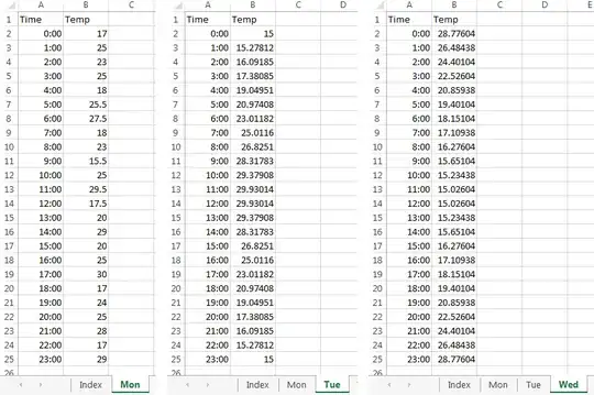
Since you haven’t given us detailed information on how your sheets are laid out, I’ll assume that you have times in cells A2:A25 and temperatures in cells B2:B25 on each of your daily sheets, like this:

On your Index sheet, enter

In A1, “Day”. (This is just a label; the same as you have shown in your image of your desired result).
In B1, your drop-down list of the days of the week.
In J1, “Time”. (This is just a label, and is optional.)
In K1, “Temp”. (This is just a label, and is optional.)
In L1, =B1 & " Temp". This will be the chart title.
In J2:J25, the times 00:00 through 23:00. Or, if some sheets have different “X”-axis values (for example, if some days have 00:30 through 23:30), enter
```
=IF(INDIRECT($B$1&"!A"&ROW())<>"", INDIRECT($B$1&"!A"&ROW()), "")
```

in J2 and drag/fill down to J25 (assuming that you always have 24 data points). You may need to manually format this correctly (e.g., hh:mm). This will access time data (i.e., X-axis labels) from Column A of the indexed daily sheet, forcing empty cells to be treated as blank rather than zero (see Display Blank when Referencing Blank Cell in Excel).

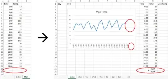
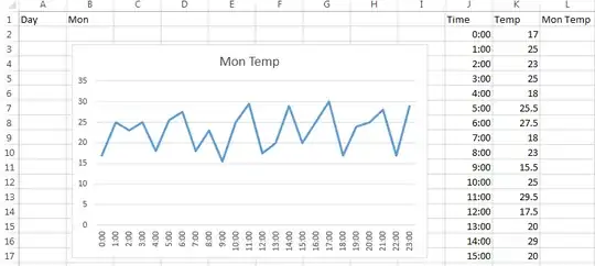
In K2, =IF(INDIRECT($B$1&"!B"&ROW())<>"", INDIRECT($B$1&"!B"&ROW()), #N/A). This will access temperature data from Column B of one of the daily sheets, replacing empty cells with #N/A (the “not available” pseudo-value), which will cause the corresponding data points not to be included in the chart. Select K2 and drag/fill down to K25. The temperature data for the selected day will appear.

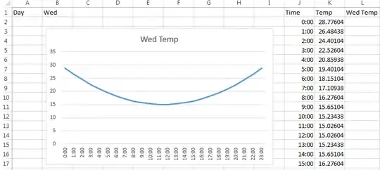
Now create your chart based on J1:K25 of the Index sheet. Click on the chart title, and type =Index!L1 into the formula bar. Then simply select the day that you want in Index!B1, and the chart for that day’s data will automatically, immediately appear — no need to press a button.

Sample result with missing data:

Of course the choice of cells is arbitrary. I used Columns J through L so I could fit them on the page with the chart. If you’d rather not see the selected data, use Columns AA through AC so they’ll be out of sight — and/or hide the auxiliary columns.

busybyte · Answer 2 · 2019-03-09T03:48:18.790

This is a vba macro, updating the chart-data. Without error-checking and most names for a better understanding

Private Sub SetChart(sheetChrt as worksheet, sheetData as worksheet)
 With sheetChrt.ChartObjects(1).Chart.SeriesCollection(1)
   .XValues = sheetData.Range("A1:A10") '
   .Values = sheetData.Range("B1:B10")
 End With
End Sub

Public Sub Test1()
 with Thisworkbook
 SetChart .Sheets("MyChartSheet"), .Sheets("MyDataSheet")
 end with
End Sub

How can I select data and draw chart using a button in Excel?

2 Answers2