Display Blank when Referencing Blank Cell in Excel 2010

Question

I have an Excel 2010 workbook that contains a number of individual worksheets. The cells on one of the sheets are linked to individual cells on two other worksheets in the same workbook. I'm using a direct cell reference that essentially says that whatever value is entered into a particular cell on one sheet also populates cells on two other sheets. I used the (=) function with the cell reference to accomplish this.

The issue I'm running into is that, even when the primary cell is left blank, the cells that populate from that primary cell will display 0, rather than remaining blank themselves.

I want the subordinate cells to remain blank if the primary cell they're linked to is blank.

wbeard52 · Answer 1 · 2015-10-30T23:38:51.437

63

You need to force Excel to treat the contents of the cell as a text value instead of a number, which it does automatically with blank values.

=A2 & ""

This will force Excel into making that cell reference a text value, thus preventing the conversion of blanks into zeroes.

edited Oct 30 '15 at 23:38

answered Apr 28 '15 at 04:56

wbeard52

3,483

Scott - Слава Україні · Answer 2 · 2012-12-06T21:35:38.953

Here are three answers:

1) Letting other.cell.reference represent the reference formula that you currently have after the = (e.g., Sheet17!$H$42), replace that link reference with

=IF(other.cell.reference<>"",other.cell.reference, "")

2) Set the “Number” format of your linked cells to “Custom”: General;–General;.

3) In “Excel Options”, “Advanced” page, “Display options for this worksheet” section, clear the “Show a zero in cells that have a zero value” checkbox. Warning: this will cause all zeroes in the worksheet to disappear.

rayzinnz · Answer 3 · 2015-04-28T22:54:12.410

IF your reference data is only either a numeric type (non-text) or empty, and you may have 0's, then this is my preferred approach, with only entering formula once. Admittedly, a slightly indirect way, but it is best I think because:

you don't need extra cells to put the formula in and then reference the second cells
you don't need to type the formula twice
this method differentiates between a zero value and an empty cell
doesn't require VBA
doesn't require Named Ranges

Downfall: If you need text data returned this this will not work. For text data my preferred method is using number format as mentioned in other answers above.

=IFERROR((A1 & "") * 1,"")

A1 in this instance can be replaced by any cell, including another sheet, workbook, or INDIRECT().

Notes on how this works:
IFERROR() - second argument is set to empty string, so if an error occurs we get an empty string. So we need to make sure if the source cell is empty, an error is triggered.

Numeric method: Stringify the source value, then multiply by 1. Literal emtpy string * 1 = #VALUE, String with numeric is auto-converted to numeric and no error occurs.

score 5 · Answer 4 · edited May 23 '17 at 12:41

5

There is another trick: set the soucre empty cell to formula ="". See the detailed description here.

edited May 23 '17 at 12:41

Community

1

answered Jun 08 '15 at 10:22

Aleksey F.

151

score 2 · Answer 5 · edited Jun 22 '17 at 13:00

2

Solution for Excel 2010:

Open "File"
Press "Options"
Click "Advanced"
Under "Display Options" for this worksheet "BBBB"
Untick the box "Show a zero value for cells that have a zero value."

edited Jun 22 '17 at 13:00

styrofoam fly

1,886

answered Jun 22 '17 at 12:20

C.B.MISRA

21

score 2 · Answer 6 · answered Jul 25 '14 at 12:35

I too did not find a better solution than the Scott's one.

But combined with the approach from here it could be almoste bearable, I think:

http://www.ozgrid.com/Excel/named-formulas.htm

Let's say I have formula like this

= IFERROR( INDEX(INDIRECT("EsZkouska");
  SMALL(IF((INDEX(INDIRECT("EsZkouska");;1‌;1)="ČSN721180")*(INDEX(INDIRECT("EsZkouska");;9;1)="RC_P_B");
  ROW(INDIRECT"EsZkouska"))-MIN(ROW(INDIRECT("EsZkouska")))+1;"");1);17;1);"")

This formula reads cell value from a data sheet using conditional select and presents them on another sheet. I have no control over cell formating on the data sheet.

I go to Insert > Name > Define and in the "Names in workbook" I create new Name "RC_P_B". Then into the "Refers to" field I copy my formula (without {} characters - it is array formula).

Then you can use Scott's formula whithout having to repeat the whole formula text:

 {=IF(RC_P_B<>""; RC_P_B;"---")}

I believe this is better than to copy the whole formula.

score 2 · Answer 7 · answered Nov 09 '14 at 06:28

2

I simple don't use a formula to overcome this problem. All I do is to conditionally format cells to font color white if cell value equals 0.

answered Nov 09 '14 at 06:28

Firas

21

score 1 · Answer 8 · answered Feb 21 '24 at 23:29

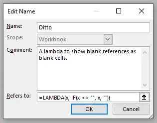
If you have a newer version of Excel that supports lambdas, you can write one as follows:

Define a new name in the Name Manager, say, Ditto.
In the Refers to: field, type =LAMBDA(x, IF(x <> "", x, "")).
Hit OK to save the lambda.
Use Ditto as a regular function; e.g., =Ditto(A5) will copy the contents of A5 but leave a blank as blank.

This method appears to work regardless of cell type or formatting. It's similar to =IF(A5 = "", "", A5), a method I've used for years, but shorter and less prone to typos.

Brad Patton · Answer 9 · 2012-12-06T21:55:05.670

1

If the linked cell is non-numeric you can use an IF statement with ISTEXT:

=IF(ISTEXT(Sheet1!A2), Sheet1!A2, "")

edited Dec 06 '12 at 21:55

answered Dec 06 '12 at 21:30

Brad Patton

10,668

score 1 · Answer 10 · answered Jun 11 '15 at 03:35

I have long searched for an elegant solution to this issue.

I have used formula =if(a2="","",a2) for years, but I find it to be a bit cumbersome.

I tried above suggestion =a2&"" and although it does appear to work it shows a number that is actually text so number formatting cannot be applied and no statistical operations work, such as sum, average, median, etc., so if it's workable numbers you're looking for this doesn't fit the bill.

I experimented with some of the other functions and found what I think is the most elegant solution to date. Continuing the above example:

=CELL("contents",A2)

returns a numerical value that can be formatted as a number and it returns a blank when the referenced cell is blank. For some reason, this solution doesn't seem to appear in any of the online suggestions I've found, but it

score 0 · Answer 11 · edited Jan 08 '16 at 17:49

0

Public Function FuncDisplayStringNoValue(MyCell As Variant) As String

Dim Result As Variant

If IsEmpty(MyCell) Then

   FuncDisplayStringNoValue = "No Value"

Else
   Result = CDec(MyCell)

   Result = Round(Result, 2)

   FuncDisplayStringNoValue = "" & Result

   End If

End Function

edited Jan 08 '16 at 17:49

nKn

5,832

answered Jan 08 '16 at 17:33

Ramon Salazar

1

score 0 · Answer 12 · edited Jan 29 '18 at 14:55

0

I have a solution working for me:

IF(cell reference="","",cell reference)

Explanation:

"" is equal to blank or empty cell. Now I only turn the if around. If cell is blank, make it blank, otherwise use the cell reference.

edited Jan 29 '18 at 14:55

Pierre.Vriens

1,425

answered Jan 29 '18 at 12:01

Sebastian Tidare

11

score 0 · Answer 13 · answered Apr 22 '18 at 16:42

0

I used conditional formatting to format the font to be the same color as the cell background where the cell value was equal to zero.

answered Apr 22 '18 at 16:42

Butonic

1

score 0 · Answer 14 · answered Jan 12 '24 at 08:58

0

You can use the expression =IF(ISBLANK(Ref Cell),"",Ref Cell)

If you have a long expression, use the following format: =IF(Ref Cell<>"",Ref Cell, "")

answered Jan 12 '24 at 08:58

Swaraj Kumar

1

score 0 · Answer 15 · answered Feb 22 '24 at 01:21

I'm surprised no one has mentioned this method:

=IF(ISBLANK(A1),TEXT(A1,"#"),A1)

Essentially the same trick as changing the data format, but this method is formulaec and thus you can preserve the cell data format type and only output a blank cell in the case that the source cell is blank; therefore, having a legitimate "0" in the source cell will still output a "0" as the output.

score -1 · Answer 16 · answered Jul 15 '15 at 15:20

I had a similar problem, and I think I found a method for you. It fixed my issues.

If you want column C to reference column A, and only write a formula for the reference cell, you would use this and drag down the column.

=A1

However, there may be source cells in column A that are blank and need to remain blank in the reference cells in column C, you can use this and drag the down column.

=T(A1)

As far as cell formatting goes, the reference (columnn C) will need to be general.

score -2 · Answer 17 · edited Nov 30 '15 at 08:44

Solution:
=IF('Wk1 Data-replace w dt bgn & end'!C2>0, 'Wk1 Data-replace w dt bgn & end'!C2, "")

Explanation:
To solve this problem I used two sets of If commands.

Part one of command:
I told the cell to display the contents of the reference cell if the reference cell contained data (Excel interprets this as the cell having a value larger than 0)

Part two of command:
I told it how to behave if there was no data; "" means leave blank

Note: Wk1 Data-replace w dt bgn & end'!C2 is my reference cell.

score -2 · Answer 18 · answered Aug 13 '16 at 21:40

-2

All these solutions are way too complicated for me and I realize this may not be a feasible for all applications but I just fill the source field with a blank and i get a blank in the destination field.

answered Aug 13 '16 at 21:40

John Alonso

1

score -2 · Answer 19 · edited Mar 18 '15 at 03:51

-2

What worked for me in Office 2013 was:

=IF(A2=""," ",A2)

Where on the first set of quotations there is no space, and on the second set there is a space.

Hope this helps

edited Mar 18 '15 at 03:51

Sathyajith Bhat

62,374

answered Mar 17 '15 at 20:24

Andy

1

score -2 · Answer 20 · edited Sep 25 '15 at 21:07

-2

Go to Format Cells.

Then select custom format, and enter the following: 0;-0;;@

edited Sep 25 '15 at 21:07

G-Man Says 'Reinstate Monica'

8,029

answered Sep 25 '15 at 19:33

Avik

1

Display Blank when Referencing Blank Cell in Excel 2010

20 Answers20

Linked

Related