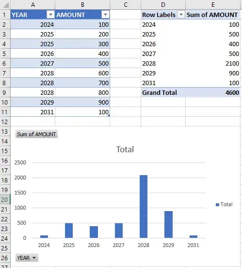
I have a table in Excel 2016:
     YEAR_     AMOUNT
---------- ----------
      2024        100
      2025        200
      2025        300
      2026        400
      2027        500
      2028        600
      2028        700
      2028        800
      2029        900
      2031        100
I'm using the table in a PivotTable and a PivotChart (bar chart):
That works, but I need bars for each year within this range: system year + 9. In other words, I want bars for 10 years, starting with the current year (currently 2023).
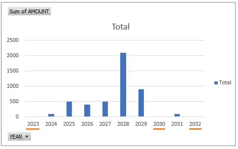
So I need to force Excel to show empty bars for 2023, 2030, and 2032.
It would look like this:
How can I force the bar chart to show the missing years? I'm looking for a dynamic solution; I don't want to manually enter filler rows into the table.
Related:

