OpenSCAD User Manual/Other Language Features

These are three of the Special Variables defined as part of the language.

Best Practice: Set $fs=0.5, $fa=1, $fn=0 for good smooth curves with reasonable performance and only use $fn > 0 to generate regular polygons.

The $fa, $fs values, OR the $fn value, are used to calculate how many facets a curved line or surface should be divided into, creating line segments or polygons respectively, to approximate a smoothed curve.

Smoothness Notes

• The terms fragment and facet are used interchangeably in this section.
• When $fn > 0, $fs and $fa are not used, and vice versa
• the number of facets is always an integer value.

These smoothness variables are actually involved in the generation of geometry, not rendering per se. Of course the generation of polygonal approximations of the mathematical shapes modeled by a script is pretty close to the rendering process. Just without rendering an image or exporting an STL file to be 3D printed.

Including this section in the Rendering page is a reflection of it being a source of rendering issues.

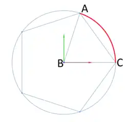
When $fa and $fs variables are being used curved objects are divided into a minimum of 5 fragments.

$fa is the minimum angle for a fragment, the angle A-B-C in the diagram, and controls the division of large circles. The minimum angle prevents a large circle being divided into microscopic facets that can't be rendered or a reproduced on a 3D printer. The default value is 12 which gives 30 fragments around a circle. The minimum value allowed is 0.01.

$fs is the minimum size of a fragment, measured in millimeters along its arc length, from A to C (in red) and controls the division of small circles. The minimum arc length prevents a circle being divided into microscopic sides, as for $fa. The default value is 2 so very small circles have a smaller number of fragments than specified using $fa. The minimum allowed value is 0.01.

The radius of curvature is factored into the fragments calculation so best practice recommendation of $fa=1 and $fs=0.5 produces smooth looking curves for a very wide range of size.

When greater than zero, $fn is an integer value setting the number of fragments that a curved line or surface will be divided into, to a minimum of 3. When assigned a floating point value any fractional part is truncated, thus $fn=6.89 results in 6-sided objects.

Curves will appear to be smoother as $fn is increased, but will require more memory and CPU power to render. Setting $fn >= 128 is not recommended.

Best Practice: is to only use $fn to create regular polygonal shapes, leaving curve smoothness to $fa and $fs. low values for $fn may be used to create regular polygons or 3D prisms

When the $fn value is divisible by 4 the polygon will be drawn on integral boundaries and be inscribed within a circle of the given diameter.

The curved 3D objects, spheres and cylinders, are divided into pie-shaped facets in the same way as circles are, and are also divided into horizontal "slices" using a similar calculation. Then, between the vertices formed by the divisions four sided polygons are drawn. The tops and bottoms are drawn as polygons with the same number of edges as there are facets.

This subdivision method is used on curved, regular shapes imported from DXF files, but is not used on 3D shapes from STL files as they are already in triangles.

This is the C code that calculates the number of fragments for a circle of radius "r":

 int get_fragments_from_r(double r, double fn, double fs, double fa)
     {
     if (r < GRID_FINE)
         return 3;
     if (fn > 0.0)
         return (int)(fn >= 3 ? floor(fn) : 3); // minimum 3
                  // which ever of $fa or $fs is used, minimum 5
     return (int) ceil( fmax( fmin( 360.0 / fa, r*2*M_PI / fs), 5 ) );
     }

GRID_FINE is an arbitrary constant for the smallest radius that will be accepted as an argument to the primitive generating object modules.

This is the equivalent calculation in OpenSCAD given a radius (r) for the curve:

 r=10; // radius of the curve being considered
 echo(
   n=($fn>0?
       ($fn>=3? $fn : 3) : 
       ceil( max( min( 360/$fa, r*2*PI/$fs ), 5 ) )
       ),
   a_based = 360/$fa,
   s_based = r*2*PI/$fs
   );
 ECHO: n = 30, a_based = 30, s_based = 31.4159

The curvature variables may be set globally in a program:

$fs = 3.1;
sphere(2);

or individually set on a primitive as a named parameter:

sphere(2, $fn = 6.4);

or modified by a scaling factor taking advantage of local scope rules:

sphere( 2, $fa = $fa*1.1 );

These Special Variables reflect the current viewport parameters at the time of rendering.

The current viewport values may be copied onto the clipboard using the menu items Edit > Copy Viewport *. From there it may be pasted into a script.

Changing the view interactively does not affect the special variables. During an animation they are updated for each frame.

$vpr

rotation vector of floats [phi-x,phi-y,phi-z] - Camera Pan, Tilt & Yaw

$vpt

translation vector [x,y,z] - Camera Rack, Truck & Pedestal

$vpf

non-negative float > 5, - Camera Zoom, set as the angle in degrees of the Field of View (FoV) [Note: Requires version 2021.01]

$vpd

non-negative float > 0.01, the camera distance [Note: Requires version 2015.03]

These four variables give the position and orientation of the camera, or eye point, that is used as the basis for rendering images.

The effect of rotation on the camera must always factor in the cameras base position and its distance.

With rotation set to [0,0,0] and translate=[0,0,0] the view is down the Z axis to the origin. The camera's rotation is clockwise, considered looking from the origin in the positive direction of the axis, so [0,90,0] rotates the camera "down" to the X axis, still looking at the origin.

Rotations are applied at the translated position of the camera and will appear to be reversed by the change in the viewport. Rotating to move the view up means applying a rotation to tilt the camera down. Likewise, to look left the camera must rotate to the right. The effect of rotation is magnified when the Camera Distance is larger.

This sets the base position of the camera in coordinate space and is not affected by rotate and zoom. We say the base position as the camera is actually positioned the camera distance along the direction of the rotation vector from its base position.

This is the angle, in degrees, of the viewing area of the camera. Making the FoV larger does Zoom In, and smaller values Out.

A floating point value for the distance, in millimeters, from the base position to the camera, along the vector set by the rotation vector.

Example

$vpr = [0, 0, $t * 360];

causes the camera to rotate 360 degree the Z axis when animating.

Animation is started by selecting the Window > Animate menu item and then entering values for "FPS" and "Steps" in the Animation Panel that opens. The "Time" field shows the current value of $t, the animation time variable, as a decimal fraction.

This variable, when active, is used in all rotate() and translate() modules, $t*360 giving complete cycles.

The value of $t will repeat from 0 through (1 - 1/Steps). It never reaches 1 because this would produce a "hitch" in the animation if using it for rotation -- two consecutive frames would be at the same angle.

There is no variable to distinguish between the cases of animation running at the first frame ($t=0) and animation not running, so make $t=0 your rest position for the model.

Examples of Animation Scripts

[Note: Requires version 2019.05]

This Special Variable may be interrogated to know in which rendering mode the script is being run.

When in OpenCSG preview mode (F5) $preview is true. Doing a render (F6) it is false.

Tip: $fn should not be used to globally control how curved shapes are sub-divided, $fa & $fs do a better job

The render() module operates differently from either rendering mode. The value of $preview is undetermined in this snippet:

render(){
    $fn = $preview ? 12 : 72;
    sphere(r = 1);
}

The tessellation result is the same regardless.

Command Line Operation

When using the command line to render $preview is only true when exporting a PNG image. For all other forms of output ( STL, DXF, SVG, CSG, and ECHO files ) it is false. It can be forced true using the -D command line option.

Examples

$preview can be used to model in reduced detail but have fully smoothed curved surfaces the final rendered result:

FNspecial = $preview ? 12 : 72;
sphere(r = 1, $fn=FNspecial );

Best Practice: The $fn argument to the module is used so that no other shapes are affected.

Another use could be to show a complex part assembled during preview but spread out and positioned for 3D printing during rendering.

OR: When horizontal features require support in 3D printing the object may be previewed without the support structures, but rendered with them, then exported to STL for printing.

A call to echo() prints its given arguments to the compilation window (aka Console). Any number of arguments of any type may be given, including function calls and other expressions. Each given argument is separated by a comma and a space. Strings are displayed in double quotes ('"'), vectors by square brackets ("[]"), and objects inside braces ("{}").

The String Function str() may be used to prepackage a number of values into a string so that values will NOT be separated by a blank. Str() also does not add quotes around strings and does not separate elements with ", ".

Numeric values are rounded off to 5 significant digits. This means that fractions smaller than 0.000001 are not displayed and that very large values are shown in scientific notation with only the first 6 digits shown.

Arguments to Echo() may be given individual labels by using the form: 'variable=variable' as will be seem in this example.

Usage examples:

 my_h=50;
 my_r=100;
 echo("a cylinder with height : ", my_h, " and radius : ", my_r);
 echo( high=my_h, rad=my_r); // will display as high=<num> rad=<num>
 cylinder(h=my_h, r=my_r);

This example shows that the fractional part of 'b' may appear to be rounded off when printed by echo(), but is still present for use in calculations and logical comparisons:

a=1.0;
b=1.000002;
echo(a); // shows as '1'
echo(b); // also shows as '1'

if(a==b){
    echo ("a==b");
}else if(a>b){
    echo ("a>b");
}else if(a<b){
    echo ("a<b"); // will be the result
}else{
    echo ("???");
}

Shows in the Console as

ECHO: 1
ECHO: 1
ECHO: "a<b"

Echo shows very small decimal fractions, and very large values, in C Language style scientific notation.

c=1000002;
d=0.000002;
echo(c); //1e+06
echo(d); //2e-06

The syntax of values shown in this form is described in the section on [[1]]

The only control over text output by echo() is the use of '\n', '\t', and '\r' characters. These are, of course, the Escape Characters for Newline, Tab, and Return and they may be used as part of a string to, respectively, begin a new line, insert blanks to the next tab stop (every 4 spaces), and return to the beginning of the line.

HTML output is not supported in development versions, starting 2025.

[Note: Requires version 2019.05]

A call to Echo() can be made as part of an expression to print information to the console just before the expression is evaluated. This means that in when the expression includes a recursive call to a function or module that echo's arguments are shown before the recursion. To be able to see values after the expression one may use a helper function as will be shown by "result()" in the second example following.

Example

 a = 3; b = 5;
 // echo() prints values before evaluating the expression
 r1 = echo(a, b) a * b; // ECHO: 3, 5
 
 // like a let(), a call to echo() may be included as part of an expression
 r2 = let(r = 2 * a * b) echo(r) r; // ECHO: 30
 
 // use echo statement for showing results 
 echo(r1, r2); // ECHO: 15, 30

A more complex example shows how echo() can be used in both the descending and ascending paths of a recursive function.

Example printing both input values and result of recursive sum()

 v = [4, 7, 9, 12];
 function result(x) = echo(result = x) x;
 function sum(x, i = 0) = echo(str("x[", i, "]=", x[i])) result(len(x) > i ? x[i] + sum(x, i + 1) : 0);
 echo("sum(v) = ", sum(v));
 
 // ECHO: "x[0]=4"
 // ECHO: "x[1]=7"
 // ECHO: "x[2]=9"
 // ECHO: "x[3]=12"
 // ECHO: "x[4]=undef"
 // ECHO: result = 0
 // ECHO: result = 12
 // ECHO: result = 21
 // ECHO: result = 28
 // ECHO: result = 32
 // ECHO: "sum(v) = ", 32

Causes meshes to be generated for surfaces in preview mode. This improves the rendered images when the normal preview renderer produces artifacts or misses parts of the image around complex bits of geometry. An issue on GitHub discusses some of these issues, and an FAQ covers more: OpenSCAD User Manual/FAQ#Why are some parts (e.g. holes) of the model not rendered correctly?

function definition

render( convexity = 1 )

convexity

an indication to the preview renderer that objects in view are not simple. See the section on the Convexity Parameter

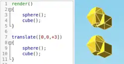
Usage examples:

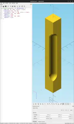
 render( convexity = 2 ) 
    difference()
        { // stretch a cube vertically
        cube([20, 20, 150], center = true);
        // make a notch in one corner 
        translate([-10, -10, 0])
            cylinder(h = 80, r = 10, center = true);
        translate([-10, -10, +40])
            sphere(r = 10);
        translate([-10, -10, -40])
            sphere(r = 10);
        }

The Surface module draws a surface based on the Height map information given either as numbers in a text data file, or by interpreting the luminance of each pixel in a PNG image file (only).

The generated surface is normally drawn from the (0,0) origin in the +X,+Y quadrant. The extent of the drawn surface is either:

• data file - the number of columns and rows in the file
• image - the number of pixels in each direction of the image.

To make a surface of size (m,n) there must be n rows of numbers, with m values on each row.

Height values from an image file are massaged to the range of 0-100 and so will not have negative values, unless the invert option changes the sign of all the height values.

Height values are applied starting at the [0,0] corner. The column index and the X coordinate are both increased by one and the next value applied at the next position on the surface. Continue like this to the end of the row and then increase the Y coordinate, and the row index, by one as the row is completed. Repeat until all the rows are processed.

For a data file of size (m,n) the generated surface is grid of squares with the height value applied at the left-lower corner (as seen here). The n-th row of heights will be on the top vertices of the squares along the top edge of the surface:

 ^  [x,y+n] [x+m,y+n]
 |
 y  [x,y]   [x+m,y]
[0,0] x-->

A one unit thick base is drawn downwards under the generated surface from the level of the smallest value in the data file, including when heights have negative values. This means that when least height value is zero the base will extend down to z=-1.

filename

Required String. The filename may include an absolute or a relative path to the height map data file. There is no default so the .png extension must be explicitly given.

center

Optional Boolean, default=false to draw in the +X,+Y quadrant. When true the surface is centered on the X-Y origin.

invert

Optional Boolean, default=false. Limitation: Only applies to image based maps

. Inverts how the pixel values are interpreted into height values.[Note: Requires version 2015.03]

convexity

Integer, default=1. Higher values improve preview rendering of complex shapes. Limitation: Only used by OpenCSG Preview

A text data height map is simply rows of whitespace separated, floating point numbers. The values may be written as integers, floating point with decimal fractions, or using exponential notation such as 1.25e2 for 125. Hex values are not accepted but may not give a warning.

Consider a data file with n rows and m values on each, thus having size (m,n). The X position of each data point is given by their position along their row, and the Y by the row. The implicit indexing starts at the beginning of the file with the first row being at Y=0 and the first point on each row at X=0. The X and Y positions increment by one until X=m and Y=n, which means that the last row of values is the farthest edge of the generated surface.

The appearance of a hash sign ('#') as the first, non-whitespace character on a line marks it as a comment. A hash mark following numbers on a row cause a lexical fault making the data file unreadable.

Examples Using Data Map

//surface.scad
surface(file = "surface.dat", center = true, convexity = 5);
%translate([0,0,5]) cube([10,10,10], center = true);

The transparent cube shows the extent of the data space, and that the base extends downwards to Y=-1.

#surface.dat
10 9 8 7 6 5 5 5 5 5 
 9 8 7 6 6 4 3 2 1 0 
 8 7 6 6 4 3 2 1 0 0
 7 6 6 4 3 2 1 0 0 0
 6 6 4 3 2 1 1 0 0 0
 6 6 3 2 1 1 1 0 0 0
 6 6 2 1 1 1 1 0 0 0
 6 6 1 0 0 0 0 0 0 0
 3 1 0 0 0 0 0 0 0 0
 3 0 0 0 0 0 0 0 0 0

Result:

One may use an application like Octave or Matlab to make a data file. This is a small Matlab script that superimposes two sine waves to create a 3D surface:

d = (sin(1:0.2:10)' * cos(1:0.2:10)) * 10;
save("-ascii", "example010.dat", "d");

The data file can then be used to draw the surface three ways:

//draw an instance of the surface
surface(file = "example010.dat", center = true);
//draw another instance, now rotated
translate(v = [70, 0, 0])
  rotate(45, [0, 0, 1])
    surface(file = "example010.dat", center = true);
// and two last instances, intersected 
translate(v = [35, 60, 0])
intersection() {
  surface(file = "example010.dat", center = true);
    rotate(45, [0, 0, 1])
      surface(file = "example010.dat", center = true);
}

[Note: Requires version 2015.03]

Heights are calculated using the linear luminance for the sRGB color space (Y = 0.2126R + 0.7152G + 0.0722B) at each pixel to derive a Grayscale value, which are further scaled to the range [0:100]. For an image with a color space between black (rgb=0,0,0) and white (rgb=1,1,1) the gray scale will be the full range.

For an image with a a narrower range of colors the gray scale is likewise reduced, and the minimum and maximum luminance in the color range set the lowest and highest limits, respectively, on the surface's heights.

Note also that no base is added below the surface as is done for a data file surface. Squares at Z=0, black, do have a surface filled in so the entire area of the surface is continuous.

Normally, with invert=false, the surface will be drawn upwards from the X-Y plane with black being z=0 increasing up to white=100. When invert=true the shape is still drawn starting at the X-Y plane, but now downwards to white=-100.

Currently only PNG (.png) images are supported and only the RGB channels are used. Specifically, the alpha channel is ignored.

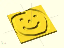
Example Using Invert

// Example 3a - apply a scale to the surface
scale([1, 1, 0.1])
  surface(file = "smiley.png", center = true);
scale([1, 1, 0.1])
  surface(file = "smiley.png", center = true, invert = true);

Input image

Example 3a: surface(invert = false)

Example 3b: surface (invert = true)

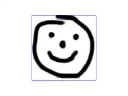
Example 3: Using surface() with a PNG image as heightmap input.

Input image

Example 4a: surface

Example 4b: surface inverted

Example 4: using a limited range PNG image.

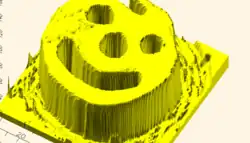
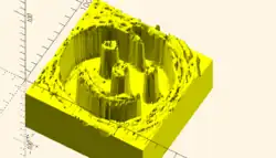
Note that the surfaces are above or, for the inverted surface, below, the X-Y plane, unlike Example 3

Example Grayscale Effects [Note: Requires version 2015.03]

surface(file = "BRGY-Grey.png", center = true, invert = false);

• 
  PNG Test File
• 
  3D Surface

The search() function is a general-purpose function to find one or more (or all) occurrences of a value or list of values in a vector, string or more complex list-of-list construct.

search( match_value , string_or_vector [, num_returns_per_match [, index_col_num ] ] );

• match_value

• Can be a single string value. Search loops over the characters in the string and searches for each one in the second argument. The second argument must be a string or a list of lists (this second case is not recommended). The search function does not search for substrings.
• Can be a single numerical value.
• Can be a list of values. The search function searches for each item on the list.
• To search for a list or a full string give the list or string as a single element list such as ["abc"] to search for the string "abc" (See Example 9) or [[6,7,8]] to search for the list [6,7,8]. Without the extra brackets, search looks separately for each item in the list.
• If match_value is boolean then search returns undef.

• string_or_vector

• The string or vector to search for matches.
• If match_value is a string then this should be a string and the string is searched for individual character matches to the characters in match_value
• If this is a list of lists, v=[[a0,a1,a2...],[b0,b1,b2,...],[c0,c1,c2,...],...] then search looks only at one index position of the sublists. By default this is position 0, so the search looks only at a0, b0, c0, etc. The index_col_num parameter changes which index is searched.
• If match_value is a string and this parameter is a list of lists then the characters of the string are tested against the appropriate index entry in the list of lists. However, if any characters fail to find a match a warning message is printed and that return value is excluded from the output (if num_returns_per_match is 1). This means that the length of the output is unpredictable.

• num_returns_per_match (default: 1)

• By default, search only looks for one match per element of match_value to return as a list of indices
• If num_returns_per_match > 1, search returns a list of lists of up to num_returns_per_match index values for each element of match_value.

• See Example 8 below.

• If num_returns_per_match = 0, search returns a list of lists of all matching index values for each element of match_value.

• See Example 6 below.

• index_col_num (default: 0)

• As noted above, when searching a list of lists, search looks only at one index position of each sublist. That index position is specified by index_col_num.
• See Example 5 below for a simple usage example.

See example023.scad included with OpenSCAD for a renderable example.

Example 5:

 data= [ ["a",1],["b",2],["c",3],["d",4],["a",5],["b",6],["c",7],["d",8],["e",3] ];
 echo(search(3, data));    // Searches index 0, so it doesn't find anything
 echo(search(3, data, num_returns_per_match=0, index_col_num=1));

Outputs:

 ECHO: []
 ECHO: [2, 8]

Example 6: Return all matches per search vector element.

 data= [ ["a",1],["b",2],["c",3],["d",4],["a",5],["b",6],["c",7],["d",8],["e",9] ];
 search("abc", data, num_returns_per_match=0);

Returns:

   [[0,4],[1,5],[2,6]]

Example 7: Return first match per search vector element; special case return vector.

 data= [ ["a",1],["b",2],["c",3],["d",4],["a",5],["b",6],["c",7],["d",8],["e",9] ];
 search("abc", data, num_returns_per_match=1);

Returns:

   [0,1,2]

Example 8: Return first two matches per search vector element; vector of vectors.

 data= [ ["a",1],["b",2],["c",3],["d",4],["a",5],["b",6],["c",7],["d",8],["e",9] ];
 search("abce", data, num_returns_per_match=2);

Returns:

 [[0,4],[1,5],[2,6],[8]]

Example 9:

 lTable2=[ ["cat",1],["b",2],["c",3],["dog",4],["a",5],["b",6],["c",7],["d",8],["e",9],["apple",10],["a",11] ];
 lSearch2=["b","zzz","a","c","apple","dog"];
 l2=search(lSearch2,lTable2);
 echo(str("Default list string search (",lSearch2,"): ",l2));

Returns

 ECHO: "Default list string search (["b", "zzz", "a", "c", "apple", "dog"]): [1, [], 4, 2, 9, 3]"

// workout which vectors get the results
v=[ ["O",2],["p",3],["e",9],["n",4],["S",5],["C",6],["A",7],["D",8] ];
//
echo(v[0]);					// -> ["O",2]
echo(v[1]);                                     // -> ["p",3]
echo(v[1][0],v[1][1]);                          // -> "p",3
echo(search("p",v));                            // find "p" -> [1]
echo(search("p",v)[0]);                         // -> 1
echo(search(9,v,0,1));                          // find  9  -> [2] 
echo(v[search(9,v,0,1)[0]]);                    // -> ["e",9]
echo(v[search(9,v,0,1)[0]][0]);                 // -> "e"
echo(v[search(9,v,0,1)[0]][1]);                 // -> 9
echo(v[search("p",v,1,0)[0]][1]);               // -> 3
echo(v[search("p",v,1,0)[0]][0]);               // -> "p"
echo(v[search("d",v,1,0)[0]][0]);               // "d" not found -> undef
echo(v[search("D",v,1,0)[0]][1]);               // -> 8

There are two functions that obtain the applications version information.

version()

returns version as a vector of three numbers [2011, 9, 23]

version_num()

returns it as a number 20110923

$parent_modules is a special variable that holds the current depth of the instantiation stack.

The parent_module(n) function returns the name of the module n levels above the module currently at the top of the instantiation stack.

Parameters

n

non-negative integer, the index of the module to get the name of. The value gives the number of steps down the stack to the module of interest. This argument should not be greater than the current value of $parent_modules.

The stack is constructed during the operation of a script, getting deeper as function or module calls create nested instances of modules, and reducing as deeper instances finish and return.

The definitions of named objects in the script(s) have nothing to do with the stack.

Example

 module top() { // define an operator module
   children();
 }
 module middle() { // define another operator module
   children();
 }
 top() 
   middle() // top of the stack, the 0-th item
     echo(parent_module(0)); // prints "middle"
 top() // 1 step down the stack
   middle()
     echo(parent_module(1)); // prints "top"

[Note: Requires version 2019.05] see also Assertion (software development)

This is a syntactic element that may be used nearly anywhere in a script. It is not a function call, does not affect scope, and cannot have a child block using braces ( "{}" ).

Assert evaluates the condition which should normally be an expression giving a Boolean result. When the result is false, the script halts and emits an error message to the console. The default report is a string showing the the expression and line number. If the second argument is given it is appended to the message.

 assert(condition)
 assert(condition, message)

Note that the appearance of assert() does not, by itself, form a statement and so no semi-colon (";") is needed to terminate it Parameters

condition

the expression given will be resolved to a Boolean true/false, if necessary using the rules for converting non-boolean values.

message

String to be appended to the message emitted when the assertion fails.

Examples

A call to assert(false); will halt the running script.

assert(false)

Emitting this message on the console

ERROR: Assertion 'false' failed in file assert_example1.scad, line 2 

Checking Parameters

// Row must draw at least 3 spheres
module row(qty) {
    assert(qty>= 3) // NOT the end of a statement
    for (i = [1 : qty])
        translate([i * 2, 0, 0]) sphere();
    }
row(0);
// ERROR: Assertion '(qty > 0)' failed in file assert_example2.scad, line 3

In cases like this using the added message can show the user how the module is intended to be used. If the assert() could be changed to:

assert(qty > 0, "Quantity must be at least 3.");

the output is more useful:

// ERROR: Assertion '(qty>=0)': "Quantity must be at least 3./" failed in file assert_example3.scad, line 2

The qty parameter can be a floating value, but by its use in the for-loop it probably should not be. The assertion can be expanded:

assert( is_num(qty) && qty >=3 )

to tighten the requirements on the input parameter

Checking Function Parameters Functions are limited to a single expression that returns a value. It is not possible to use additional if-the-else statements to test a function's given inputs but a nested ?: conditional statement avoids that restriction:

// set all letters to "lower case"
function lower(string) = 
	is_not_string( string ) ?
		undef
	: str_is_empty( string ) ?
		""
	: str_lower( string )
	;

This method has the advantage that bad inputs do not halt execution, but some may prefer a stricter enforcement of a function's interface, thusly:

// set all letters to "lower case"
function lower(string) = 
	assert( ! is_string( string ) )
	assert( string != "" )
	str_lower( string ) // does the work
	; // end of the function definition staement

If the lower() function is called with improper inputs the user will get immediate feedback.

Testing Features

To test a function that accumulates the values of an array we can set up test conditions that we know have to be correct

if(_NUMTEST_ENABLED) {
echo( "\ttesting cumsum_vec()" );
	csv = [1,3,7,1];
	vec=[ 10, 20, 30, 40 ];
	echo( cs=cumsum_vec( csv ));
	echo( cs=cumsum_vec( vec ));
	}
assert( cumsum_vec( [1,3,7,1] ) == 12 );
assert( cumsum_vec( [10, 20, 30, 40] ) == 100 );