73

I have data that looks like this:

Id | Loc1 | Loc2 | Loc3 | Loc4
---+------+------+------+-----
1  | NY   | CA   | TX   | IL
2  | WA   | OR   | NH   | RI

And I want to convert it to this:

Id | LocNum | Loc
---+--------+----
1  |   1    | NY
1  |   2    | CA
1  |   3    | TX
1  |   4    | IL
2  |   1    | WA
2  |   2    | OR
2  |   3    | NH
2  |   4    | RI

What's the easiest way to do this in Excel 2007?

shA.t
  • 500
devuxer
  • 4,111

12 Answers12

71

You can do this with a pivot table.

  1. Create a "Multiple Consolidation Ranges PivotTable." (Only on Pivot Table Wizard. Callup with ALT+D, P on Excel 2007)
  2. Select "I will create my own page fields".
  3. Select your data.
  4. Double click on the grand total value - the one at the intersection of Row Grand and Column Grand, all the way on the lower right hand corner of your pivot table.

You should see a new sheet containing all of the data in your pivot table, transposed in the way you're looking for.

Datapig technologies provides step-by-step instructions that are actually more complicated than you need - his example transposes only part of the data set & uses the pivot technique combined with TextToColumns. But it does have lots of pictures.

Note that a pivot table will group the data. If you want it ungrouped, the only way to do it is to copy the pivot table, and "paste special" as values. You can then fill in the blanks with a technique like this: http://www.contextures.com/xlDataEntry02.html

Lernkurve
  • 2,052
DaveParillo
  • 14,761
8

If your data isn't an Excel Pivot Table but just data, you might want to "un-pivot" it with some simple VBA code. The code depends on two named ranges, Source and Target. Source is the data you want to un-pivot (exclusive of the column/row headers, e.g. NY-RI in the sample) and Target is the first cell where you want to place your result.

Sub unPivot()
Dim oTarget As Range
Dim oSource As Range
Dim oCell As Range

Set oSource = Names("Source").RefersToRange
Set oTarget = Names("Target").RefersToRange

For Each oCell In oSource
    If oCell.Value <> "" Then
        oTarget.Activate
      ' get the column header
        oTarget.Value = oCell.Offset(-(oCell.Row - oSource.Row + 1), 0).Text 
      ' get the row header
         oTarget.Offset(0, 1).Value = oCell.Offset(0, _
           -(oCell.Column - oSource.Column + 1)).Text 
      ' get the value
        oTarget.Offset(0, 2).Value = oCell.Text 
      ' move the target pointer to the next row
        Set oTarget = oTarget.Offset(1, 0) 
    End If
Next
Beep
End Sub
5

I have built an add-in that will let you do that, and that makes it easy to adapt to different situations. Check it out here: http://tduhameau.wordpress.com/2012/09/24/the-unpivot-add-in/

nutsch
  • 1,971
5

There is quite a nice solution in excel 2010, just need to play a bit with pivot table.

Create a pivot table from your data with these settings:

  • no subtotals, no grand totals
  • report layout: tabular form, repeat all item labels
  • add all the columns you need, keep columns you want to transform at the right
  • for each column you want to transform: open field settings – in layout & print tab: select “Show item labels in outline form” and check both check boxes below it
  • copy your table to a separate location (just values)
  • if you have empty cells in your original data then filter for empty values in the rightmost column and delete those rows (don’t filter in pivot table as it won't work as you need!)
Jawa
  • 3,679
4

Best I've come up with so far is this:

Id   LocNum  Loc
---------------------------------
1    1       =INDEX(Data,A6,B6)
1    2       =INDEX(Data,A7,B7)
1    3       =INDEX(Data,A8,B8)
1    4       =INDEX(Data,A9,B9)
2    1       =INDEX(Data,A10,B10)
2    2       =INDEX(Data,A11,B11)
2    3       =INDEX(Data,A12,B12)
2    4       =INDEX(Data,A13,B13)

This works, but I have to generate the Id's and LocNum's manually. If there's a more automated solution (besides writing a macro), please let me know in a separate answer.

devuxer
  • 4,111
2

If the dimensions of your data are as in the sample provided in your question, then the following set of formulae using OFFSET should give you your required result:

Assuming

1 | NY | CA | TX | IL

2 | WA | OR | NH | RI

are in the range A2:E3, then enter

=OFFSET($A$2,FLOOR((ROW(A2)-ROW($A$2))/4,1),0)

in F2, say, and

=MOD(ROW(A2)-ROW($A$2),4)+1

in G2, say, and

=OFFSET($B$2,FLOOR((ROW(B2)-ROW($B$2))/4,1),MOD(ROW(A2)-ROW($A$2),4))

in H2, say.

Then copy these formulae down as far as required.

This is the easiest, pure, built-in formula solution that I can think of.

Aaa
  • 266
1

Excel has made this question easier to answer and it can be done in a single formula. It requires some newer functions such as ByRow and ByCol but these are scheduled to be available to everyone (someday).

To recap:

  • No VBA
  • Dynamic for multiple axes in both rows and columns data ranges
  • Can be converted to lambda (in desktop version)

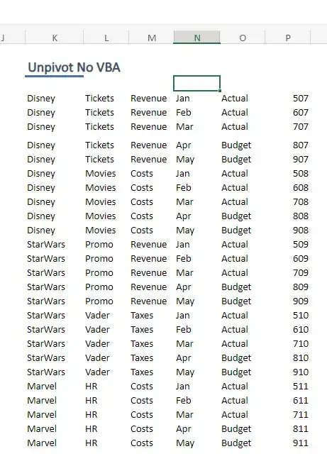
With the below dataset pasted in cell A1, you could use this Lambda function to unpivot or flatten the data:

Starting Dataset

See sample file here

(cell A1) Jan Feb Mar Apr May
Actual Actual Actual Budget Budget
Disney Tickets Revenue 507 607 707 807 907
Disney Movies Costs 508 608 708 808 908
StarWars Promo Revenue 509 609 709 809 909
StarWars Vader Taxes 510 610 710 810 910
Marvel HR Costs 511 611 711 811 911

Stand Alone Formula

=LET(dataRng,D3:H7,  rowAxis,A3:C7, colAxis,D1:H2,
   iCol,COLUMN(INDEX(rowAxis,1,1)),   amountCol,TOCOL(dataRng),  totalCells,COUNTA(amountCol),
          HSTACK(
              INDEX(rowAxis,
                     INT(SEQUENCE(totalCells,1,0,1)/COLUMNS(dataRng))+1,
                     BYCOL(INDEX(rowAxis,1,),  LAMBDA(aCol,COLUMN(aCol) -iCol +1))),
              INDEX(colAxis,
                      SEQUENCE(1,ROWS(colAxis),1,1),
                      MOD(SEQUENCE(totalCells,1,0,1),COLUMNS(dataRng))+1),
               amountCol))

Lambda Formula

=LAMBDA(dataRng,rowAxis,colAxis,
   LET(iCol,COLUMN(INDEX(rowAxis,1,1)), amountCol,TOCOL(dataRng), totalCells,COUNTA(amountCol),
          HSTACK(
              INDEX(rowAxis,
                     INT(SEQUENCE(totalCells,1,0,1)/COLUMNS(dataRng))+1,
                     BYCOL(INDEX(rowAxis,1,),  LAMBDA(aCol,COLUMN(aCol) -iCol +1))),
              INDEX(colAxis,
                      SEQUENCE(1,ROWS(colAxis),1,1),
                      MOD(SEQUENCE(totalCells,1,0,1),COLUMNS(dataRng))+1),
               amountCol
                      )))(D3:H7,A3:C7,D1:H2)

enter image description here

Also, if you did happen to want a vba solution, I used to use this:

Function unPivotData(theDataRange As Range, theColumnRange As Range, theRowRange As Range, _
    Optional skipZerosAsTrue As Boolean, Optional includeBlanksAsTrue As Boolean, Optional columnsFirst As Boolean)

'Set effecient range Dim cleanedDataRange As Range Set cleanedDataRange = Intersect(theDataRange, theDataRange.Worksheet.UsedRange)

'tests Data ranges

'Use intersect address to account for users selecting full row or column

If cleanedDataRange.EntireColumn.Address <> Intersect(cleanedDataRange.EntireColumn, theColumnRange).EntireColumn.Address Then unPivotData = "datarange missing Column Ranges"

ElseIf cleanedDataRange.EntireRow.Address <> Intersect(cleanedDataRange.EntireRow, theRowRange).EntireRow.Address Then unPivotData = "datarange missing row Ranges"

ElseIf Not Intersect(cleanedDataRange, theColumnRange) Is Nothing Then unPivotData = "datarange may not intersect column range. " & Intersect(cleanedDataRange, theColumnRange).Address

ElseIf Not Intersect(cleanedDataRange, theRowRange) Is Nothing Then unPivotData = "datarange may not intersect row range. " & Intersect(cleanedDataRange, theRowRange).Address

End If

'exits if errors were found If Len(unPivotData) > 0 Then Exit Function

Dim dimCount As Long dimCount = theColumnRange.Rows.Count + theRowRange.Columns.Count

Dim aCell As Range, i As Long, g As Long, tangoRange As Range ReDim newdata(dimCount, i)

'loops through data ranges For Each aCell In cleanedDataRange.Cells

If aCell.Value2 = "" And Not (includeBlanksAsTrue) Then 'skip ElseIf aCell.Value2 = 0 And skipZerosAsTrue Then 'skip Else ReDim Preserve newdata(dimCount, i) g = 0

'gets DimensionMembers members
    If columnsFirst Then
        Set tangoRange = Union(Intersect(aCell.EntireColumn, theColumnRange), _
            Intersect(aCell.EntireRow, theRowRange))
      Else
       Set tangoRange = Union(Intersect(aCell.EntireRow, theRowRange), _
       Intersect(aCell.EntireColumn, theColumnRange))
    End If

    For Each gcell In tangoRange.Cells
        newdata(g, i) = IIf(gcell.Value2 = &quot;&quot;, &quot;&quot;, gcell.Value)
        g = g + 1
    Next gcell

         newdata(g, i) = IIf(aCell.Value2 = &quot;&quot;, &quot;&quot;, aCell.Value)
         i = i + 1
End If

Next aCell

unPivotData = WorksheetFunction.Transpose(newdata) End Function

1

There is a parametric VBA conversion utility to unpivot or reverse pivoted data back to a database table, please see

http://www.spreadsheet1.com/unpivot-data.html

Petros
  • 11
1

Here is a nice tool to unpivot, normalize a Pivot Table.

Normalisieren von Pivot Tabellen

I hope it helps.

Excellll
  • 12,847
1

You seem to have gotten the "loc" column (evidenced by your first answer), and now you need help getting the other two columns.

Your first option is to simply type the first several (say, 12) rows into those columns and drag down - I think Excel does the right thing in this case (I don't have excel on this computer to test it for sure).

If that doesn't work, or if you want something more programmer-y, try using the row() function. Something like "=Floor(row()/4)" for the ID column and "=mod(row(),4)+1" for the LocNum column.

1

@DaveParillo answer is the best answer for a single tab table. I wanted to add some extras here.

For Multiple columns pre the unpivot columns

This method does not work.

Youtube unpivot simple data like the question

This is a youtube video showing how to do it in a simple manner. I skipped the part about adding the shortcut and used @devuxer shortcut that is in DaveParillo answer.

https://www.youtube.com/watch?v=pUXJLzqlEPk

-3

It's much simple than this. Just click the "Transpose" option in "Paste Special..." to get the transposition you are requesting.

jonsca
  • 4,084