OpenSCAD User Manual/The OpenSCAD Language
Chapter 1 -- General
OpenSCAD User Manual/The OpenSCAD Language Scripts in the OpenSCAD language are functional descriptions of how a designer's intent may realized in a solid model.
Program Structure
The statement is the basis of the language:
<perform named operations>;
The end of a statement is marked by a literal semi-colon (';').
Each statement either :
- assigns the result of an expression to a variable
- invokes one or more modules to instantiate a shape that appears in the preview panel
- modifies the script's flow of execution.
Evaluating Expressions
Expressions are evaluated before any module in a statement.
The evaluation of an expression results in a value of a specific type and may replace a single variable or literal wherever syntax requires a value.
When used in a simple statement the result must be assigned to a variable
<Named Variable> = <expression>;
but in general the result of an expression is used immediately as a syntactic element.
- for( <loop variable> = <condition> ) <statement>
- [vector] = [for( <loop variable> = [<start>:<incr>:<end>] ) make_list_element( <loop variable> ) ]
- make_shape( <param>, <name>=<param> )
- echo( "giving feedback", <function_under_test>( <param> ) );
where <condition>, the <start>:<incr>:<end> values in the range, each parameter value in the call to the module, and the <function_under_test>, and <param> may all be expressions.
Modules are Parents
Modules are not like the subroutines that are the building blocks of procedural languages. OpenSCAD is all about constructing a model out of solid geometry elements, and has been designed to organize it elements in parent-child relationships.
Syntactically, the first module in a statement is a parent, and all following modules are its children. Likewise, every child is parent to any modules following them in a statement.
parent() { child(); child() { grandson() ggchild(); granddaughter() } }
The built-in modules are implemented without the ability to have children, meaning they should appear last in a statement. But user-defined modules may draw shapes and accept child modules().
Module parent-child structures may be created in the statements that are part of an If-Then-Else or For-Loop and vice versa:
module xx() {
    sphere();
    children();
    }

xx() for(i=[1,3]) translate([i*2,0,0]) cube();
This works because the xx module used a call to children() to "register" that it will accept the "responsibilities" of parenthood.
Note: Any flow of control or module following a built-in module will emit a warning and do nothing else. The module will draw its shape, but cannot handle children.
Constructing Solid Geometry
The normal operation of Constructive Solid Geometry (CSG) is to form complex shapes by combining primitive and derived shapes and performing operations on them.
To create a shape an Object Module is called:
make_shape();
where "make_shape()" is a user defined module, but equally represents a call to any of the built-in modules. The built-in modules have default values for their parameters and will draw an appropriate shape using them when called with an empty argument list.
Note: data structure objects have been added to the language as of the 2025.07.* development snapshot releases. To clarify the language of this document, modules make curves and shapes, not objects. Only the object() function can create data structures of the object type.
To manipulate or modify an object any number of Operator Modules may be called before the make_shape():
operator() make_shape();
operator() operator() make_shape();
It is important to understand that the ability to act as parent, child, or both is part of the implementation of the "module" in OpenSCAD.
That said, it is convenient to treat the built-in modules as being of two types, operators, and shape builders, as a consequence of their implementation, as explained in the section on writing user-defined modules.
2D Shapes and Extrusion
Any of the 2 Dimensional Primitives, Polygons, Text, and Imported 2D shapes may be the basis for extrusions that create 3D shapes.
3D Shapes and Combinations
Any of the 3 Dimensional Primitives, Polyhedrons, and Imported 3D Shapes may be the basis for Boolean Combinations that create 3D shapes. It is also possible to project a 3D shape onto a coordinate place to obtain its 2D silhouette.
Structure and Scope
Normally a statement does just one thing, and for assignment expressions that is enough. The choice between alternatives in an if-then-else, or the body of a for-loop, often need to perform more than one operation. OpenSCAD borrows the lexical structure of other programming languages to extend a single statement into a block of them.
A block of statements is created using braces to mark the beginning and end of the block:
{
operator() object();
operator() object();
}
This simple block is not much use as such, but it shows that any single statement may be replaced by a block of statements inside a pair of braces.
A better illustration would be:
{
for(...) { // A
    make_shape_1();
    if(...) then { // B
       operator() make_shape_2();
       operator() make_shape_3();
       } // end B
    else
       make_other_shape()
    } // end A
}
There is an overlap between the previously mentioned parent-child relations between modules and the lexical structure of this last example. Although the outer for-loop is not a module, its body being a block of statements means that it has children, the shapes drawn by make_shape_1() and the if-then-else. And that, further, it has grandchildren ... either two when the <condition> expression is true, or just one if false.
Flow Of Control
As with any structured programming language decision making and looping statements are critical features of OpenSCAD scripts. In a functional language the path, or flow, of execution through the code is controlled by the FoC statements.
The statements available are the if(cond)-else and the for([range]) loop. FoC statements are written to operate on single statements, thusly:
if(<condition>) <when true do this statement>;
else <when false do this statement>;
and with looping
for(i=[0:9]) object(); // make 10 objects
A more readable example:
if( is_string(s) )
    operator() object(file=s); // do this when <condition> == true
else
    object(file="default.dat"); // otherwise do this
Of course a single statement is often not enough. Different statement types and use cases have these coping mechanisms:
- When the statement is an assignment expression the calculation may be written into a function as calling a function is a valid expression.
- A sequence of actions may be written into a user-defined module as calling that is a single statement.
- in every case a block "{}" can replace a statement
if( is_string(s) )
    { // <condition> == true
    operator() object(file=s);
    if(<condition>)
        answer = MyOwnFunction();
    else
        answer = 12;
    }
else // <condition> == false
       // no block - the for() loop is the single statement
    for()
        { // but the target of the for loop is this block
        object(file="default.dat");
        operator() My_Own_Object();
        }
Other Uses of If and For
The for() and if() statements have an important secondary role in vector initialization, though it is not technically flow of control.
A third use of the for loop concept is special iteration_for() Operator Module for intersecting multiple instances of an object into a composite.
Again, not technically not flow of control.
Names
Named objects in OpenSCAD include Variables, Functions, and Modules.
To be valid a name:
- must begin with an alphabetic character [a..zA..Z] or an underscore ('_')
- and may continue with any mix of alphabetic characters, numeric digits, and the underscore
- and may not include accented characters, punctuation, nor Unicode characters.
Note: older versions of OpenSCAD allowed names to start with numeric digits but will generate run-time errors in more recent versions
The OpenSCAD convention on multi word names is to use the underscore to delimit them, as this_is_a_name
Variables
Named variables are created when they appear as the Left Hand Side of an assignment statement and will be given the value of the Right Hand Side expression.
result = <calculate something>;
Variables should normally be defined only once in a program as when the program runs the variable will have the last value assigned to it.
The location of a variable definition determines where it can be used, thus it has "scope", a concept discussed fully in the literature, with only a few issues germane to functional programming and OpenSCAD in particular needing to be covered in the following section.
Vectors
A vector or list is a sequence of zero or more OpenSCAD values. Vectors are collections of numeric or boolean values, variables, vectors, strings or any combination thereof. They can also be expressions that evaluate to one of these. Vectors handle the role of arrays found in many imperative languages. The information here also applies to lists and tables that use vectors for their data.
A vector has square brackets, [] enclosing zero or more items (elements or members), separated by commas. A vector can contain vectors, which can contain vectors, etc.
Examples
   [1,2,3]
   [a,5,b]
   []
   [5.643]
   ["a","b","string"]
   [[1,r],[x,y,z,4,5]]
   [3, 5, [6,7], [[8,9],[10,[11,12],13], c, "string"]
   [4/3, 6*1.5, cos(60)]
use in OpenSCAD:
  cube( [width,depth,height] );           // optional spaces shown for clarity
  translate( [x,y,z] )
  polygon( [ [x0,y0],  [x1,y1],  [x2,y2] ] );
Creation
Vectors are created by writing the list of elements, separated by commas, and enclosed in square brackets. Variables are replaced by their values.
  cube([10,15,20]);
  a1 = [1,2,3];
  a2 = [4,5];
  a3 = [6,7,8,9];
  b  = [a1,a2,a3];    // [ [1,2,3], [4,5], [6,7,8,9] ]  note increased nesting depth
Vectors can be initialized using a for loop enclosed in square brackets.
The following example initializes the vector result with a length n of 10 values to the value of a.
n = 10;
a = 0;

result = [ for (i=[0:n-1]) a ];
echo(result); //ECHO: [0, 0, 0, 0, 0, 0, 0, 0, 0, 0]
The following example shows a vector result with a n length of 10 initialized with values that are alternatively a or b respectively if the index position i is an even or an odd number.
n = 10;
a = 0;
b = 1;
result = [ for (i=[0:n-1]) (i % 2 == 0) ? a : b ];
echo(result); //ECHO: [0, 1, 0, 1, 0, 1, 0, 1, 0, 1]
Indexing elements within vectors
Elements within vectors are numbered from 0 to n-1 where n is the length returned by len(). Address elements within vectors with the following notation:
e[5]           // element no 5 (sixth) at   1st nesting level
e[5][2]        // element 2 of element 5    2nd nesting level
e[5][2][0]     // element 0 of 2 of 5       3rd nesting level
e[5][2][0][1]  // element 1 of 0 of 2 of 5  4th nesting level
e = [ [1], [], [3,4,5], "string", "x", [[10,11],[12,13,14],[[15,16],[17]]] ];  // length 6

address       length  element
e[0]          1       [1]
e[1]          0       []
e[5]          3       [ [10,11], [12,13,14], [[15,16],[17]] ]
e[5][1]       3       [ 12, 13, 14 ]
e[5][2]       2       [ [15,16], [17] ]
e[5][2][0]    2       [ 15, 16 ]
e[5][2][0][1] undef   16

e[3]          6       "string"
e[3 ][2]      1       "r"

s = [2,0,5]; a = 2;
s[a]          undef   5
e[s[a]]       3       [ [10,11], [12,13,14], [[15,16],[17]] ]
String indexing
The elements (characters) of a string can be accessed:
"string"[2] //resolves to "r"
Vector Swizzling
[Note: Requires version Dev Snapshot 2021.12.23 or later]
The components of vectors can be accessed using the following syntax:
e = [1, 2, 3, 4];
v = e.x + e.y; // yields 1 + 2 = 3
This is called swizzling. You can use x, y, z, or w, referring to the first, second, third, and fourth components, respectively. Alternatively, r, g, b, and a can be used instead of x,y,z,w.
Swizzling is named so because you can use it to repeat, reorder, or select a subset of components.
v1 = e.xyxx; // -> [1,2,1,1]
v2 = e.zyy;  // -> [3,2,2]
v3 = e.rrr;  // -> [1,1,1]
v4 = e.rg;   // -> [1,2]
You can use any combination of up to 4 of the letters to create a vector. Attempts to reference components which doesn't exist will result in an undef.
Vector Functions
concat() Function
[Note: Requires version 2015.03]
concat() combines the elements of 2 or more vectors into a single vector. No change in nesting level is made.
 vector1 = [1,2,3]; vector2 = [4]; vector3 = [5,6];
 new_vector = concat(vector1, vector2, vector3); // [1,2,3,4,5,6]

 string_vector = concat("abc","def");                 // ["abc", "def"]
 one_string = str(string_vector[0],string_vector[1]); // "abcdef"
len() Function
len() is a function that returns the length of vectors or strings.
Indices of elements are from [0] to [length-1].
- vector
- Returns the number of elements at this level.
- Single values, which are not vectors, raise an error.
- string
- Returns the number of characters in a string.
a = [1,2,3]; echo(len(a)); // 3
See example elements with lengths
Matrix
A matrix is a vector of vectors.
Example that defines a 2D rotation matrix
mr = [
     [cos(angle), -sin(angle)],
     [sin(angle),  cos(angle)]
     ];
Language Components
Most of the other commonly available components of a structured programming language are included in OpenSCAD, namely
- Named Objects and Scope
- variables, functions, and modules
- Data Types, Values, and Constants
- 64-bit floating point, boolean, string, and vector (or list)
- Data Structures
- Vectors and Objects
- Expressions
- arithmetic, string, bitwise, and logical
- Built-In Functions
- all the standard functions for use in expressions of all types
- Syntactic Operators
- The language has features that work like built-in modules but are different in detail, Echo, Let, Assert
- User Defined Objects
- custom modules and functions
Language Elements particularly needed for modelling are
- Built-in 2D Object Modules
- circle(), square(), polygon(), etc.
- 2D file import
- Adding drawn shapes from SVG, DXF, image, and text data files
- 3D File Import
- adding geometry from external sources
- Built-In 3D Object Modules
- sphere(), cube(), polyhedron(), etc.
- Built-In Operator Modules
- 3D boolean operations: intersection(), difference(), union()
- Shape Modifications : linear_extrude(), rotate_extrude(), hull(), etc.
- Transformations : translate(), rotate(), etc.
- Color
- Customizer
- Compile time user input
Values and Data Types
A value in OpenSCAD is either a Number (like 42), a Boolean (like true), a String (like "foo"), a Range (like [0: 1: 10]), a Vector (like [1,2,3]), or the Undefined value (undef). Values can be stored in variables, passed as function arguments, and returned as function results.
[OpenSCAD is a dynamically typed language with a fixed set of data types. There are no type names, and no user defined types.]
Numbers
Numbers are the most important type in OpenSCAD, and they are written in the decimal notation common to most programming languages:
- 42
- the answer for everything
- -1
- a negative value
- 0x22
- a hexadecimal value (3410)
- 0.5
- a decimal fraction
- 1.0123e-5
- a very small fraction (0.000010123) in scientific notation
- 2.99792458e+8
- a very large value in scientific notation
The internal form of numbers follows the 64-bit IEEE floating point number specification. Zero (0) and negative zero (-0) are treated as two distinct numbers by some of the math operations, and are displayed as such by 'echo', although they compare as equal. Complex numbers are not supported.
Integers are just 52-bit numbers without a fractional part. Literal hexadecimal values in a script are also evaluated to their integer value and stored as 52-bit binaries.
Values used in bitwise operations are an exception as their 64-bit encoding is binary, but only during the operation. The results of a bitwise expression are converted to the normal 64-bit floating format.
Limitation: Fractions are not represented exactly unless the denominator is a power of 2
- The largest value possible is about 1308. If an expression evaluates to a larger value it will be treated as "infinity" and printed as "inf" by echo.
- The most negative value is about -1308. Negative infinity is printed as "-inf" by echo.
- very small fractions may be displayed as 0 or -0 by
echo().
Nearly Equal is as Close as You Get
As noted in the limitation above, power of 2 fractions, like 0.25 (1/4) and 0.375 (3/8), are represented exactly, but 2 divided by 10, 2/10 = 0.2 is only approximated.
Also, 64-bit floating values are only accurate to 15-17 decimal digits, meaning that the least significant digit of a 17 digit number is undetermined.
In practice this means that two FP values calculated differently, but that should come to same result, may encoded to slightly different digits, which will cause a test for equality to fail. This happens when their differences are close to, or less than, the Min.Normal value derived from the numerical representation (see geekley's list of Number Limits).
A Quick and Dirty solution to the Nearly Equal problem is to see if the difference of the two values is smaller than an acceptable value, epsilon.
/**	returns true when two floating point values are within
  epsilons value of each other. */
function _nearly_equal( a, b, epsilon=0.00001 ) =
    abs(( a - b )/ b ) < epsilon
    ;
A more elegant, and more numerically correct version is available in the numbers.scad file of the relativity library (soon to be released), provided here as an extract from the library.
Hexadecimal Literals
C style hexadecimal constants are allowed to be assigned to variables.
hex1 = 0x32;     // ASCII space
hex2 = 0x98 - 1; // ASCII 'a'
num1 = 0x2334;   // 9012
num2 = 0x233411  // 2.30709e+6
[Note: Requires version Development snapshot].
OpenSCAD does not support octal notation for numbers.
Predefined Numeric Constants
These special numbers are defined:
PI- π, 3.141592 approximately. The ratio between the diameter and circumference of a circle.
infinities- there is no constant for
infnor-inf NaN- Not a Number, nor is
nana real constant.
While there are no constants for inf, -inf, and nan they can be created by arithmetic operations and be assigned to variables for when needed:
inf = 1e200 * 1e200;
nan = 0 / 0;
echo(inf,nan); // ECHO: inf, nan
As mentioned at the top of this page, the 64-bit encoding of floating point values requires that both positive and negative infinity have to be able to be displayed in output messages.
To be able to display something for undefined math results, like or Divide by Zero the industry "standard" is "Not A Number", or nan.
The background for this issue is covered at the Open Group's site on math.h and the page on the IEEE 754 staqndard.

OpenSCAD has not implemented everything as it is in C/C++. For example, it uses degrees angles and trigonometric functions. This table shows the results of giving undefined inputs to built-in math functions taken from the regression test suite in 2015.
| 0/0: nan | sin(1/0): nan | asin(1/0): nan | ln(1/0): inf | round(1/0): inf |
| -0/0: nan | cos(1/0): nan | acos(1/0): nan | ln(-1/0): nan | round(-1/0): -inf |
| 0/-0: nan | tan(1/0): nan | atan(1/0): 90 | log(1/0): inf | sign(1/0): 1 |
| 1/0: inf | ceil(-1/0): -inf | atan(-1/0): -90 | log(-1/0): nan | sign(-1/0): -1 |
| 1/-0: -inf | ceil(1/0): inf | atan2(1/0, -1/0): 135 | max(-1/0, 1/0): inf | sqrt(1/0): inf |
| -1/0: -inf | floor(-1/0): -inf | exp(1/0): inf | min(-1/0, 1/0): -inf | sqrt(-1/0): nan |
| -1/-0: inf | floor(1/0): inf | exp(-1/0): 0 | pow(2, 1/0): inf | pow(2, -1/0): 0 |
Testing for NaN
The value nan is the only OpenSCAD value that is not equal to any other value, including itself.
The conditional expression x == 0/0 will fail with a run-time error.
Instead, you must use 'x != x' to test if x is "nan".
The Undefined Value
The undefined value is a special value written as undef. It is the initial value of a variable that hasn't been assigned a value, and it is often returned as a result by functions or operations that are passed illegal arguments. Finally, undef can be used as a null value, equivalent to null or NULL in other programming languages.
All arithmetic expressions containing undef values evaluate as undef. In logical expressions, undef is equivalent to false. Relational operator expressions with undef evaluate as false except for undef==undef, which is true.
Note that numeric operations may also return 'nan' (not-a-number) to indicate an illegal argument. For example, 0/false is undef, but 0/0 is 'nan'. Relational operators like < and > return false if passed illegal arguments. Although undef is a language value, 'nan' is not.
Variables cannot be changed
A variable is created by the assignment statement that sets its value, thus defining it, and it cannot thereafter be changed. But, unlike constants in other languages, assignments may be overridden.
A second assignment to the same variable will cause a warning about its value being reassigned, and has the effect of replacing first assignment with the second one. In fact, the value that the variable holds throughout the run-time of the script is that set by the last assignment that uses it as the LHS.
a = 1;   // effectively replaced and never executed
echo(a); // 2
a = 2;   // as if executed at the a=1 statement
echo(a); // 2
There are two exceptions to this behavior:
- an assignment in an included file may be given a new value in the including file.
- an assignment in a script will take a new value from
-Dcommand line option - likewise for a variable set in the Customizer.
This allows variables to be given default values in a shared library that are then given new values in scripts that include it.
// main.scad
include <lib.scad>
a = 2;
echo(b); // ECHO: 3
// lib.scad
a = 1;
b = a + 1;
Run-Time Data Sources
An OpenSCAD program cannot prompt the user for interactive input while running, but it is possible to access data from files, the Customizer Panel, and the command line.
- the Customizer may be used to set values that modify the parsing and rendering of an .scad program
- If the app is opened from the command line a
-Dat the-D valueargument - read data from .stl, .dxf, or .png files.
Import Objects from STL Files
OpenSCAD can import objects from STL files to be manipulated (translation, clipping, etc.) and rendered. The data in the STL file cannot be accessed.
Access Data in DXF Files
Data in a DXF file may be accessed using this functions:
- [X,Y,Z] = dxf_cross( file="name.dxf", layer="a.layer", origin=[0,0], scale=1.0 )
- This function returns the intersection of two lines on the given layer.
- N= dxf_dim( file="name.dxf", name="namedDimension", layer="a.layer", origin=[0, 0], scale=1);
Function dxf_cross()
The function looks for two lines on the given layer and calculates their intersection. The intersection may not be defined as a point entity.
OriginPoint = dxf_cross(file="drawing.dxf", layer="SCAD.Origin",
                        origin=[0, 0], scale=1);
Function dxf_dim()
Dimensions in a DXF file that are named may be accessed for use in an OpenSCAD program using a call to dxf_dim();
TotalWidth = dxf_dim(file="drawing.dxf", name="TotalWidth",
                        layer="SCAD.Origin", origin=[0, 0], scale=1);
DXF File Data Access Example
For a nice example of both functions, see Example009 and the image on the homepage of OpenSCAD.
Chapter 2 -- 3D Objects
OpenSCAD User Manual/The OpenSCAD Language
Primitive Solids
Cube() Object Module
Creates a cube or rectangular prism (i.e., a "box") in the first octant. When center is true, the cube is centered on the origin. Argument names are optional if given in the order shown here.
cube(size = [x,y,z], center = true/false);
cube(size =  x ,     center = true/false);
- parameters:
- size
- single value, cube with all sides this length
- 3 value array [x,y,z], rectangular prism with dimensions x, y and z.
- center
- false (default), 1st (positive) octant, one corner at (0,0,0)
- true, cube is centered at (0,0,0)
- size
default values: cube(); yields: cube(size = [1, 1, 1], center = false);
- examples:
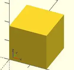
equivalent scripts for this example
 cube(size = 18);
 cube(18);
 cube([18,18,18]);
 .
 cube(18,false);
 cube([18,18,18],false);
 cube([18,18,18],center=false);
 cube(size = [18,18,18], center = false);
 cube(center = false,size = [18,18,18] );
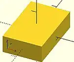
equivalent scripts for this example
 cube([18,28,8],true);
 box=[18,28,8];cube(box,true);
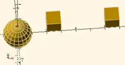
Sphere() Object Module
With default parameters this module draws a unit sphere at the origin of the coordinate system, centered vertically on the X-Y plane. It appears as a five sided polyhedron when $fn is zero per the smoothness variables.
default sphere( 1, $fn = 0, $fa = 12, $fs = 2 )
Parameters
- 1) r
- non-negative float, radius
- d
- non-negative float, diameter
- $fn, $fs, $fa
- Smoothness settings, see Rendering: Curve_Smoothness
Radius
The distance from the sphere's center to its surface. A negative value will emit a warning and draw nothing. The smoothness of the surface is determined by the smoothness parameters, $fn, $fs, $fa
Diameter
This must be given as a named parameter.
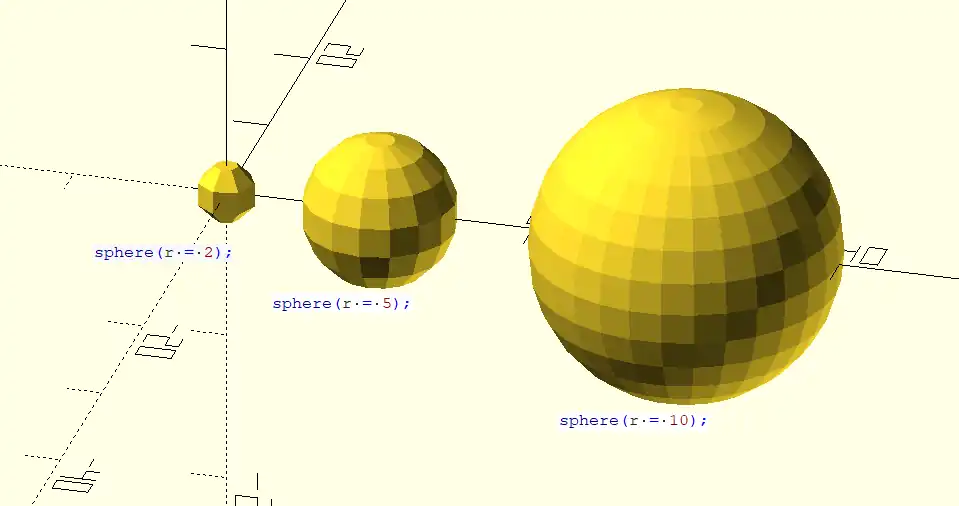
Usage Examples
sphere();       // radius = 1 by default
sphere(r = 2);
sphere(d = 4);  // same size as previous
To draw a very smooth sphere with a 2 mm radius:
sphere(2, $fn=100);
// also creates a 2mm high resolution sphere but this one
// does not have as many small triangles on the poles of the sphere
sphere(2, $fa=5, $fs=0.1);
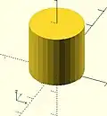
Cylinder() Object Module
Creates a cylinder or cone centered about the z axis.
Called with no arguments, and $fn at its default, the module creates a 1 unit tall, pentagonal solid on the X-Y plane that is inscribed in a unit circle.
Parameter names are optional if the first three are given in the order of height, radius 1 (bottom radius), and radius 2 (top radius) as seen here:
cylinder(h, r1, r2);
Omitting r1 or r2 leaves them at their default values of one resulting in a truncated cone (a Conical Frustum). The named parameters may be given in any order, but for any of the diameter related ones only the first given is used. Giving a diameter/radius value of zero results in a cone shape, and setting both to zero make no shape at all.
- Parameters
- h : (pos 1) height of the cylinder, must be greater than zero
- r1 : (pos 2) radius of bottom circular face.
- r2 : (pos 3) radius of top circular face.
- center : (pos 4)
- false (default), height is from the X-Y plane to positive Z
- true height is centered vertically on the X-Y plane
- r : radius of both end faces
- d : diameter of both end faces. [Note: Requires version 2014.03]
- d1 : diameter of bottom circular face. [Note: Requires version 2014.03]
- d2 : diameter of top circular face. [Note: Requires version 2014.03]
- $fa : minimum angle (in degrees) of each fragment.
- $fs : minimum circumferential length of each fragment.
- $fn : fixed number of fragments in 360 degrees. Values of 3 or more override $fa and $fs
- $fa, $fs and $fn must be named parameters. click here for more details,.
default values:
 cylinder($fn = 0, $fa = 12, $fs = 2, h = 1, r1 = 1, r2 = 1, center = false);
 cylinder($fn = 0, $fa = 12, $fs = 2, h = 1, d1 = 1, d2 = 1, center = false); // radius = 0.5
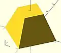
All of the following calls result in this conic frustum:

cylinder(h=15, r1=9.5, r2=19.5, center=false);
cylinder(  15,    9.5,    19.5, false);
cylinder(  15,    9.5,    19.5);
cylinder(  15,    9.5, d2=39  );
cylinder(  15, d1=19,  d2=39  );
cylinder(  15, d1=19,  r2=19.5);
All of these result in this cone:

cylinder(h=15, r1=10, r2=0, center=true);
cylinder(  15,    10,    0,        true);
cylinder(h=15, d1=20, d2=0, center=true);
-
 center = false
 -
 center = true
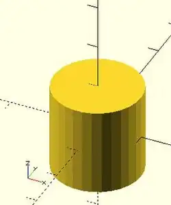
equivalent scripts
 cylinder(h=20, r=10, center=true);
 cylinder(  20,   10, 10,true);
 cylinder(  20, d=20, center=true);
 cylinder(  20,r1=10, d2=20, center=true);
 cylinder(  20,r1=10, d2=2*10, center=true);
- use of $fn
Larger values of $fn create smoother surfaces at the cost of greater rendering time. A good practice is to set it in the range of 10 to 20 during development of a shape, then change to a value larger than 30 for rendering image or exporting shape files.
However, use of small values can produce some interesting non circular objects. A few examples are show here:


scripts for these examples
 cylinder(20,20,20,$fn=3);
 cylinder(20,20,00,$fn=4);
 cylinder(20,20,10,$fn=4);
- undersized holes
Using cylinder() with difference() to place holes in objects creates undersized holes. This is because circular paths are approximated with polygons inscribed within in a circle. The points of the polygon are on the circle, but straight lines between are inside. To have all of the hole larger than the true circle, the polygon must lie wholly outside of the circle (circumscribed). Modules for circumscribed holes
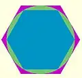
script for this example
 poly_n = 6;
 color("blue") translate([0, 0, 0.02]) linear_extrude(0.1) circle(10, $fn=poly_n);
 color("green") translate([0, 0, 0.01]) linear_extrude(0.1) circle(10, $fn=360);
 color("purple") linear_extrude(0.1) circle(10/cos(180/poly_n), $fn=poly_n);
In general, a polygon of radius has a radius to the midpoint of any side as . If only the midpoint radius is known (for example, to fit a hex key into a hexagonal hole), then the polygon radius is .


Polyhedron() Object Module
A polyhedron is the most general 3D primitive solid. It can be used to create any regular or irregular shape including those with concave as well as convex features. Curved surfaces are approximated by a series of flat surfaces.
polyhedron( points = [ [X0, Y0, Z0], [X1, Y1, Z1], ... ], triangles = [ [P0, P1, P2], ... ], convexity = N);   // before 2014.03
polyhedron( points = [ [X0, Y0, Z0], [X1, Y1, Z1], ... ], faces = [ [P0, P1, P2, P3, ...], ... ], convexity = N);   // 2014.03 & later
Parameters
- points
- vector of [x,y,z] vertices. Points may be defined in any order.
- triangles
- [Deprecated: triangles will be removed in a future release. Use Use
facesparameter instead instead] Vector of triangles that enclose the solid. Triangles are vectors containing three indices into the points vector.
- faces
- [Note: Requires version 2014.03] Vector of faces that collectively enclose the solid. Each face is a vector containing the indices (0 based) of 3 or more points from the points vector. Faces may be defined in any order, but the points of each face must be ordered correctly (see below). Define enough faces to fully enclose the solid, with no overlap. If points that describe a single face are not on the same plane, the face is automatically split into triangles as needed.
- convexity
- Integer, default=1
Facing and Points Order
In the list of faces, for each face it is arbitrary which point you start with, but the points of the face (referenced by the index into the list of points) must be ordered in clockwise direction when looking at each face from outside inward. The back is viewed from the back, the bottom from the bottom, etc.
Another way to remember this ordering requirement is to use the left-hand rule. Using your left hand, stick your thumb up and curl your fingers as if giving the thumbs-up sign, point your thumb away from the face, and order the points in the direction your fingers curl (this is the opposite of the STL file format convention, which uses a "right-hand rule"). Try this on the example below.
Example 1
Using polyhedron to generate a rectangular prism [ 10, 7, 5 ] :
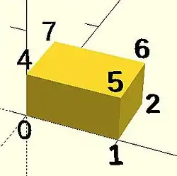
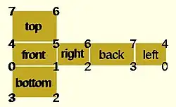
CubePoints = [
  [  0,  0,  0 ],  //0
  [ 10,  0,  0 ],  //1
  [ 10,  7,  0 ],  //2
  [  0,  7,  0 ],  //3
  [  0,  0,  5 ],  //4
  [ 10,  0,  5 ],  //5
  [ 10,  7,  5 ],  //6
  [  0,  7,  5 ]]; //7

CubeFaces = [
  [0,1,2,3],  // bottom
  [4,5,1,0],  // front
  [7,6,5,4],  // top
  [5,6,2,1],  // right
  [6,7,3,2],  // back
  [7,4,0,3]]; // left

polyhedron( CubePoints, CubeFaces );
equivalent descriptions of the bottom face
  [0,1,2,3],
  [0,1,2,3,0],
  [1,2,3,0],
  [2,3,0,1],
  [3,0,1,2],
  [0,1,2],[2,3,0],   // 2 tris with no overlap
  [1,2,3],[3,0,1],
  [1,2,3],[0,1,3],
- Example 2 A square base pyramid:
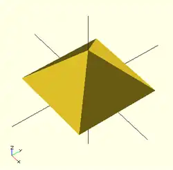
polyhedron(
  points=[ [10,10,0],[10,-10,0],[-10,-10,0],[-10,10,0], // the base
           [0,0,10]  ],                       // the apex point
  faces=[ [0,1,4],[1,2,4],[2,3,4],[3,0,4],    // each triangle side
          [1,0,3],[2,1,3] ]                   // two triangles for square base
 );
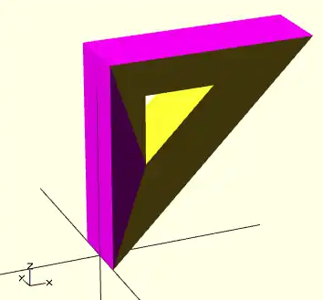
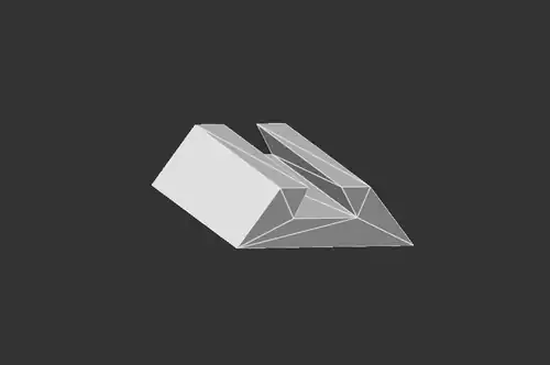
Example 3 A triangular prism
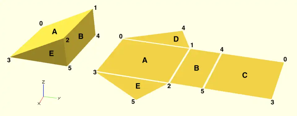
module prism(l, w, h) {
    polyhedron(// pt      0        1        2        3        4        5
               points=[[0,0,0], [0,w,h], [l,w,h], [l,0,0], [0,w,0], [l,w,0]],
               // top sloping face (A)
               faces=[[0,1,2,3],
               // vertical rectangular face (B)
               [2,1,4,5],
               // bottom face (C)
               [0,3,5,4],
               // rear triangular face (D)
               [0,4,1],
               // front triangular face (E)
               [3,2,5]]
               );}
prism(10, 10, 5);
Debugging Polyhedra
Mistakes in defining polyhedra include not having all faces in clockwise order (viewed from outside - a bottom need to be viewed from below), overlap of faces and missing faces or portions of faces. As a general rule, the polyhedron faces should also satisfy manifold conditions:
- exactly two faces should meet at any polyhedron edge.
- if two faces have a vertex in common, they should be in the same cycle face-edge around the vertex.
The first rule eliminates polyhedra like two cubes with a common edge and not watertight models; the second excludes polyhedra like two cubes with a common vertex.
When viewed from the outside, the points describing each face must be in the same clockwise order, and provides a mechanism for detecting counterclockwise. When the thrown together view (F12) is used with F5, CCW faces are shown in pink. Reorder the points for incorrect faces. Rotate the object to view all faces. The pink view can be turned off with F10.
OpenSCAD allows, temporarily, commenting out part of the face descriptions so that only the remaining faces are displayed. Use // to comment out the rest of the line. Use /* and */ to start and end a comment block. This can be part of a line or extend over several lines. Viewing only part of the faces can be helpful in determining the right points for an individual face. Note that a solid is not shown, only the faces. If using F12, all faces have one pink side. Commenting some faces helps also to show any internal face.
CubeFaces = [
/* [0,1,2,3],  // bottom
   [4,5,1,0],  // front */
   [7,6,5,4],  // top
/* [5,6,2,1],  // right
   [6,7,3,2],  // back */
   [7,4,0,3]]; // left
After defining a polyhedron, its preview may seem correct. The polyhedron alone may even render fine. However, to be sure it is a valid manifold and that it can generate a valid STL file, union it with any cube and render it (F6). If the polyhedron disappears, it means that it is not correct. Revise the winding order of all faces and the two rules stated above.
Mis-ordered faces
Example 4
a more complex polyhedron with mis-ordered faces When you select 'Thrown together' from the view menu and compile (preview F5) the design (not compile and render!) the preview shows the mis-oriented polygons highlighted. Unfortunately this highlighting is not possible in the OpenCSG preview mode because it would interfere with the way the OpenCSG preview mode is implemented.)
Below you can see the code and the picture of such a problematic polyhedron, the bad polygons (faces or compositions of faces) are in pink.
// Bad polyhedron
polyhedron
    (points = [
	       [0, -10, 60], [0, 10, 60], [0, 10, 0], [0, -10, 0], [60, -10, 60], [60, 10, 60],
	       [10, -10, 50], [10, 10, 50], [10, 10, 30], [10, -10, 30], [30, -10, 50], [30, 10, 50]
	       ],
     faces = [
		  [0,2,3],   [0,1,2],  [0,4,5],  [0,5,1],   [5,4,2],  [2,4,3],
                  [6,8,9],  [6,7,8],  [6,10,11], [6,11,7], [10,8,11],
		  [10,9,8], [0,3,9],  [9,0,6], [10,6, 0],  [0,4,10],
                  [3,9,10], [3,10,4], [1,7,11],  [1,11,5], [1,7,8],
                  [1,8,2],  [2,8,11], [2,11,5]
		  ]
     );
A correct polyhedron would be the following:
polyhedron
    (points = [
	       [0, -10, 60], [0, 10, 60], [0, 10, 0], [0, -10, 0], [60, -10, 60], [60, 10, 60],
	       [10, -10, 50], [10, 10, 50], [10, 10, 30], [10, -10, 30], [30, -10, 50], [30, 10, 50]
	       ],
     faces = [
		  [0,3,2],  [0,2,1],  [4,0,5],  [5,0,1],  [5,2,4],  [4,2,3],
                  [6,8,9],  [6,7,8],  [6,10,11],[6,11,7], [10,8,11],
		  [10,9,8], [3,0,9],  [9,0,6],  [10,6, 0],[0,4,10],
                  [3,9,10], [3,10,4], [1,7,11], [1,11,5], [1,8,7],
                  [2,8,1],  [8,2,11], [5,11,2]
		  ]
     );
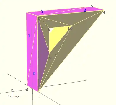
Face Orientation in Polyhedra
If you don't really understand "orientation", try to identify the mis-oriented pink faces and then invert the sequence of the references to the points vectors until you get it right. E.g. in the above example, the third triangle ([0,4,5]) was wrong and we fixed it as [4,0,5]. Remember that a face list is a circular list. In addition, you may select "Show Edges" from the "View Menu", print a screen capture and number both the points and the faces. In our example, the points are annotated in black and the faces in blue. Turn the object around and make a second copy from the back if needed. This way you can keep track.
- Clockwise technique
Orientation is determined by clockwise circular indexing. This means that if you're looking at the triangle (in this case [4,0,5]) from the outside you'll see that the path is clockwise around the center of the face. The winding order [4,0,5] is clockwise and therefore good. The winding order [0,4,5] is counter-clockwise and therefore bad. Likewise, any other clockwise order of [4,0,5] works: [5,4,0] & [0,5,4] are good too. If you use the clockwise technique, you'll always have your faces outside (outside of OpenSCAD, other programs do use counter-clockwise as the outside though).
Think of it as a "left hand rule":
If you place your left hand on the face with your fingers curled in the direction of the order of the points, your thumb should point outward. If your thumb points inward, you need to reverse the winding order.
Succinct description of a 'Polyhedron'
- Points define all of the points/vertices in the shape.
- Faces is a list of polygons that connect up the points/vertices.
Each point, in the point list, is defined with a 3-tuple x,y,z position specification. Points in the point list are automatically enumerated starting from zero for use in the faces list (0,1,2,3,... etc).
Each face, in the faces list, is defined by selecting 3 or more of the points (using the point order number) out of the point list.
e.g. faces=[ [0,1,2] ] defines a triangle from the first point (points are zero referenced) to the second point and then to the third point.
When looking at any face from the outside, the face must list all points in a clockwise order.
Repetitions in a Point List
The point list of the polyhedron definition may have repetitions. When two or more points have the same coordinates they are considered the same polyhedron vertex. So, the following polyhedron:
points = [[ 0, 0, 0], [10, 0, 0], [ 0,10, 0],
          [ 0, 0, 0], [10, 0, 0], [ 0,10, 0],
          [ 0,10, 0], [10, 0, 0], [ 0, 0,10],
          [ 0, 0, 0], [ 0, 0,10], [10, 0, 0],
          [ 0, 0, 0], [ 0,10, 0], [ 0, 0,10]];
polyhedron(points, [[0,1,2], [3,4,5], [6,7,8], [9,10,11], [12,13,14]]);
define the same tetrahedron as:
points = [[0,0,0], [0,10,0], [10,0,0], [0,0,10]];
polyhedron(points, [[0,2,1], [0,1,3], [1,2,3], [0,3,2]]);
3D to 2D Projection
Using the projection() function, you can create 2d drawings from 3d models, and export them to the dxf format. It works by projecting a 3D model to the (x,y) plane, with z at 0. If cut=true, only points with z=0 are considered (effectively cutting the object), with cut=false(the default), points above and below the plane are considered as well (creating a proper projection).
Example: Consider example002.scad, that comes with OpenSCAD.

Then you can do a 'cut' projection, which gives you the 'slice' of the x-y plane with z=0.
projection(cut = true) example002();

You can also do an 'ordinary' projection, which gives a sort of 'shadow' of the object onto the xy plane.
projection(cut = false) example002();

Another Example
You can also use projection to get a 'side view' of an object. Let's take example002, rotate it, and move it up out of the X-Y plane:
translate([0,0,25]) rotate([90,0,0]) example002();
Now we can get a side view with projection()
projection() translate([0,0,25]) rotate([90,0,0]) example002();

Links:
- More complicated example from Giles Bathgate's blog
Chapter 3 -- 2D Objects
OpenSCAD User Manual/The OpenSCAD Language All 2D primitives can be transformed with 3D transformations. They are usually used as part of a 3D extrusion. Although they are infinitely thin, they are rendered with a 1-unit thickness.
Note: Trying to subtract with difference() from 3D object will lead to unexpected results in final rendering.
Square Object Module
By default this module draws a unit square in the first quadrant, (+X,+Y), starting at the origin [0,0]. Its four lines have no thickness but the shape is drawn as a 1 unit high, filled plane.
The module's arguments may be written in the order <size>, center=<bool> without being named, but the names may be used as shown in the examples:
Parameters
- size
- has two forms: single value or vector
- single - non-negative float, length of all four sides
- array[x,y] of two non-negative floats, the length of the sides in the x and y directions
- center
- boolean, default false, to set the shape's position in the X-Y plane
Center
When false, as it is by default, the shape will be drawn from its first point at (0,0) in the First Quadrant, (+X,+Y).
With center set to true the shape is drawn centered on the origin.
Examples
Except for being 10 cm square this is a default square:
 square(size = 10, center=false);
 square(10,false);
 square([10,10]);

And to draw a 20x10 rectangle, centered on the origin, like this:
 square([20,10],true);
 a=[20,10]; square(a,true);

Circle Object Module
By default this module draws a unit circle centered on the origin [0,0] as a pentagon with its starting point on the X-axis at X=1. Its lines have no thickness but the shape is drawn as a 1 unit high, filled plane.
The circle() shape is drawn as if inscribed in a circle of the given radius, starting at a point on the positive x axis.
The argument radius may be given without being named, but the r and d arguments must be named.
Parameters
- 1) radius
- non-negative float, radius of the circle
- r
- non-negative float, radius of the circle
- d
- non-negative float, diameter of the circle
- $fa
- Special Variable
- $fs
- Special Variable
- $fn
- Special Variable
The default circle displays as a pentagram as that is the minimum number of fragments used to approximate a curved shape calculated from the default values for $fs and $fa. To have it draw as a smooth shape increase the $fn value, the minimum number of fragments to draw, to 20 or more (best $fn < 128).
An alternative method to draw a very smooth circle scale is to scale down a very large circle.
scale( 0.001 ) circle(200);

Equivalent scripts for this example
 circle(10);
 circle(r=10);
 circle(d=20);
Drawing an Ellipse
There is no built-in module that for generating an ellipse, but the scale() or resize() operator modules may be used to form an ellipse.
See OpenSCAD User Manual/Transformations
Examples
resize([30,10]) circle(d=20); // change the circle to X and Y sizes

scale([1.5,0.5]) circle(d=20); // apply X and Y factors to circle dimensions

Regular Polygons
There is no built-in module for generating regular polygons.
It is possible to use the special variable $fn rendering parameter to set the number of sides to use when drawing the circle().
circle(r=1, $fn=4); // generate a unit square
Examples
The following script draws these these examples:

translate([-42,  0])
    {circle(20,$fn=3);  %circle(20,$fn=90); }
translate([  0,  0]) circle(20,$fn=4);
translate([ 42,  0]) circle(20,$fn=5);
translate([-42,-42]) circle(20,$fn=6);
translate([  0,-42]) circle(20,$fn=8);
translate([ 42,-42]) circle(20,$fn=12);

color("black"){
    translate([-42,  0,1])text( "3",7);
    translate([  0,  0,1])text( "4",7);
    translate([ 42,  0,1])text( "5",7);
    translate([-42,-42,1])text( "6",7);
    translate([  0,-42,1])text( "8",7);
    translate([ 42,-42,1])text("12",7);
    }
Another way to solve the lack of a built-in module for regular polygons is to write a custom one: module regular_polygon()
Polygon Object Module
The polygon() module draws lines between the points given in a vector of [x,y] coordinates using, optionally, one or more "paths" that specify the order of the points to draw lines between, overriding the "natural" order. Polygons are always created in the X-Y plane and are co-planar by definition.
A polygon is the most general of the 2D objects in that it may be used to generate shapes with both concave and convex edges, have interior holes, and effectively perform boolean operations between shapes defined by paths.
Note that the order of the points sets how the lines will be drawn so complex shapes made with crossing lines can be achieved without using a path argument, but making interior holes do require the use of at least two paths to set the interior and exterior boundary lines.
The determination of which parts of the polygon to fill and to leave empty is handled automatically and it is only the filled parts that will be extruded, if the shape will be used as a basis for that operation. Note also that a shape drawn entirely within a "hole" will be filled in, and any shape its interior will again be a hole, and so on.
polygon(points, paths = undef, convexity = 1);
Parameters
- points
- required and positional - A vector of [x,y] coords that define the points of the polygon
- paths
- optional, default=undef - a vector of vectors of indices into the points vector with no restrictions on order or multiple references.
- convexity
- Integer, default=1 - complex edge geometry may require a higher value value to preview correctly.
Points Parameter A list of X-Y coordinates in this form:
[[1, 1], [1, 4], [3, 4], [3, 1], [1, 1]]
which defines four points and makes it explicit that the last one is the same as the first.
Including the first point twice is not strictly necessary as this:
[[1, 1], [1, 4], [3, 4], [3, 1]]
gives the same result.
Paths Parameter
This optional parameter is a nested vector of paths.
A "path" is a list of index values that reference points in the points vector.
It can explicitly describe a closed loop by its last index being the same as its first, as in:
[1, 2, 3, 4, 1]
but this is equivalent to:
[1, 2, 3, 4]
Paths that cross each other can implicitly perform boolean operations but to cut holes in the interior of the polygon paths will have to be used.
Notice that the points vector is simple list, while each path is a separate vector. This means that paths, that are lists of references to points, have to "know" which points it needs to include. This can be an issue if the polygon is assembled from a number of shapes at run time as the order of adding shapes affects their point's index values. . Convexity
Shapes with a lot of detail in their edges may need the convexity parameter increased to preview correctly. See Convexity
Example With No Holes
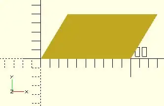
This will draw a slanted rectangle:
polygon(points=[[0,0],[100,0],[130,50],[30,50]]);
and the same shape with the path vector:
polygon([[0,0],[100,0],[130,50],[30,50]], paths=[[0,1,2,3]]);
Note that the path can index the points starting with any one of them, so long as the list of references "walks" around the outside of the shape.
Example With One Hole
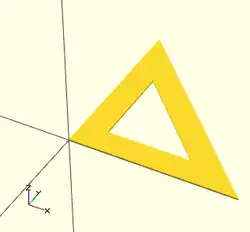
Using vector literals to draw a triangle with its center cut out. Note the two paths:
polygon(
   [[0,0],[100,0],[0,100],[10,10],[80,10],[10,80]],
   [[0,1,2],[3,4,5]]
   );
And using variables:
triangle_points =[[0,0],[100,0],[0,100],[10,10],[80,10],[10,80]];
triangle_paths =[[0,1,2],[3,4,5]];
polygon(triangle_points,triangle_paths);
When there is a shape wholly inside the bounds of another it makes a hole.
Example With Multiple Holes
[Note: Requires version 2015.03] (for use of concat())
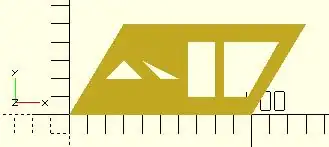
We are using "a" for the point lists and "b" for their paths:
a0 = [[0,0],[100,0],[130,50],[30,50]];     // outer boundary
b0 = [1,0,3,2];
a1 = [[20,20],[40,20],[30,30]];            // hole 1
b1 = [4,5,6];
a2 = [[50,20],[60,20],[40,30]];            // hole 2
b2 = [7,8,9];
a3 = [[65,10],[80,10],[80,40],[65,40]];    // hole 3
b3 = [10,11,12,13];
a4 = [[98,10],[115,40],[85,40],[85,10]];   // hole 4
b4 = [14,15,16,17];
a  = concat( a0,a1,a2,a3,a4 ); // merge all points into "a"
b  = [b0,b1,b2,b3,b4]; // place all paths into a vector
polygon(a,b);
      //alternate
polygon(a,[b0,b1,b2,b3,b4]);
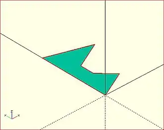
2D to 3D by Extrusion
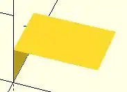
A polygon may be the basis for an extrusion, just as any of the 2D primitives can. This example script may be used to draw the shape in this image:
Import a 2D Shape From a DXF
[Deprecated: import_dxf() will be removed in a future release. Use Use import() Object Module instead. instead]
Read a DXF file and create a 2D shape.
Example
linear_extrude(height = 5, center = true)
		import_dxf(file = "example009.dxf", layer = "plate");
Example with Import()
linear_extrude(height = 5, center = true)
		import(file = "example009.dxf", layer = "plate");
Text in OpenSCAD
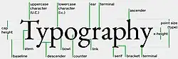
Being able to use text objects as a part of a model is valuable in a lot of design solutions. The text() module is used to draw a string of text as a set of 2D shapes according to the specifications of the given font. The fonts available to use in a script are from the system that OpenSCAD is running in with the addition of those explicitly added by the script itself. To be able to format text, or to align text in relation to other shapes, a script needs information about the text objects that the script is working on, and also about the structure and dimensions of the fonts in use.
text() Object Module
The text() object module draws a single string of text as a 2D geometric object, using fonts installed on the local system or provided as separate font file.
The shape starts at the origin and is drawn along the positive X axis.
Vertical alignment, as set by the valign parameter, is relative to the X axis, and horizontal alignment ( halign ) to the Y axis
[Note: Requires version 2015.03]
Parameters
- text
- String. A single line of any character allowed. Limitation: non-printable ASCII characters like newline and tab rendered as placeholders
- font
- a formatted string with default font of "Liberation Sans:style=Regular"
- size
- non-negative decimal, default=10. The generated text has a height above the baseline of approximately this value, varying for different fonts but typically being slightly smaller.
- halign
- String, default="left". The horizontal alignment for the text. Possible values are "left", "center" and "right".
- valign
- String, default="baseline". The vertical alignment for the text. Possible values are "top", "center", "baseline" and "bottom".
- spacing
- float, default=1. Multiplicative factor that increases or decreases spacing between characters.
- direction
- String, default="ltr". Direction of text. Possible values are "ltr" (left-to-right), "rtl" (right-to-left), "ttb" (top-to-bottom) and "btt" (bottom-to-top).
- language
- String. The language of the text (e.g., "en", "ar", "ch"). Default is "en".
- script
- String, default="latin". The script of the text (e.g. "latin", "arabic", "hani").
- $fn
- higher values generate smoother curves (refer to Special Variables)
Example
_example.png)
text("OpenSCAD");
Font & Style Parameter
The "name" of a font is a string starting with its logical font name and variation, optionally followed by a colon (":") separated list of font specifications like a style selection, and a set of zero or more features.
The common variations in a font family are sans and serif though many others will be seen in the list of fonts available.
Each font variation can be drawn with a style to support textual emphasis.
The default, upright appearance is usually called "Regular" with "Bold", "Italic", and "Bold Italic" being the other three styles commonly included in a font. In general the styles offered by a font may only be known by using the platform's font configuration tools or the OpenSCAD font list dialog.
_font_features_example.png)
In addition to the main font variations, some fonts support features for showing other glyphs like "small-caps" (smcp) where the lower case letters look like scaled down upper case letters, or "old-numbers" (onum) where the numbers are designed in varying heights instead of the way modern lining draws numbers the same size as upper case letters.
The fontfeatures property is appended to the font name after the optional style parameter.
Its value is a semi-colon separated list of feature codes, each prefixed by a plus, "+", to indicate that it is being added,
font = "Linux Libertine G:style=Regular:fontfeatures=+smcp;+onum");
Basic Font Parameter Example
_font_style_example.png)
 square(10);

 translate([15, 15]) {
   text("OpenSCAD", font = "Liberation Sans");
 }

 translate([15, 0]) {
   text("OpenSCAD", font = "Liberation Sans:style=Bold Italic");
 }
Size Parameter
Text size is normally given in points, and a point is 1/72 of an inch high.
The formula to convert the size value to "points" is pt = size/3.937, so a size argument of 3.05 is about 12 points.
Note: Character size the distance from ascent to descent, not from ascent to baseline.
Vertical Alignment
One of these four names must be given as a string to the valign parameter.
- top
- The text is aligned so the top of the tallest character in your text is at the given Y coordinate.
- center
- The text is aligned with the center of the bounding box at the given Y coordinate. This bounding box is based on the actual sizes of the letters, so taller letters and descending below the baseline will affect the positioning.
- baseline
- The text is aligned with the font baseline at the given Y coordinate. This is the default, and is the only option that makes different pieces of text align vertically, as if they were written on lined paper, regardless of character heights and descenders.
- bottom
- The text is aligned so the bottom of the lowest-reaching character in your text is at the given Y coordinate.
Note: only the "baseline" vertical alignment option will ensure correct alignment of texts that use mix of fonts and sizes.
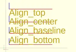
 text = "Align";
 font = "Liberation Sans";

 valign = [
   [  0, "top"],
   [ 40, "center"],
   [ 75, "baseline"],
   [110, "bottom"]
 ];

 for (a = valign) {
   translate([10, 120 - a[0], 0]) {
     color("red") cube([135, 1, 0.1]);
     color("blue") cube([1, 20, 0.1]);
     linear_extrude(height = 0.5) {
       text(text = str(text,"_",a[1]), font = font, size = 20, valign = a[1]);
     }
   }
 }
Horizontal Alignment
One of these three names must be given as a string to the halign parameter.
- left
- The text is aligned with the left side of the bounding box at the given X coordinate.
- center
- The text is aligned with the center of the bounding box at the given X coordinate.
- right
- The text is aligned with the right of the bounding box at the given X coordinate.
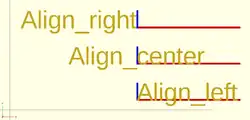
 text = "Align";
 font = "Liberation Sans";

 halign = [
   [10, "left"],
   [50, "center"],
   [90, "right"]
 ];

 for (a = halign) {
   translate([140, a[0], 0]) {
     color("red") cube([115, 2,0.1]);
     color("blue") cube([2, 20,0.1]);
     linear_extrude(height = 0.5) {
       text(text = str(text,"_",a[1]), font = font, size = 20, halign = a[1]);
     }
   }
 }
Spacing Parameter
Characters in a text element have the size dictated by their glyph in the font being used.
As such their size in X and Y is fixed.
Each glyph also has fixed advance values (it is a vector [a,b], see textmetrics) for the offset to the origin of the next character.
The position of each following character is the advance.x value multiplied by the space value.
Obviously letters in the string can be stretched out when the factor is greater than 1, and can be made to overlap when space is a fraction closer to zero, but interestingly, using a negative value spaces each letter in the opposite of the direction parameter.
Text Examples
Simulating Formatted Text
When text needs to be drawn as if it was formatted it is possible to use translate() to space lines of text vertically.
Fonts that descend below the baseline need to be spaced apart vertically by about 1.4*size to not overlap.
Some word processing programs use a more generous spacing of 1.6*size for "single spacing" and double spacing can use 3.2*size.
Fonts in OpenSCAD
The fonts available for use in a script are thosed:
- registered in the local system
- included in the OpenSCAD installation
- imported at run-time by a program
A call to fontmetrics() using only default settings shows the installation's standard font and settings:
echo( fontmetrics() );
gives this output (formatted for readability)
{
nominal = {
  ascent = 12.5733;
  descent = -2.9433;
  };
max = {
  ascent = 13.6109; descent = -4.2114;
  };
interline = 15.9709;
font = {
  family = "Liberation Sans";
  style = "Regular";
  };
}
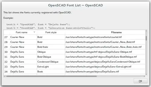
In general the styles offered by a font may only be known by using the platform's font configuration tools or the OpenSCAD font list dialog.
The menu item Help > Font List shows the list of available fonts and the styles included in each one.
None of the platforms OpenSCAD is available on include the Liberation font family so having it as part of the app's installation, and making it the default font, avoids problems of font availability. There are three variations in the family, Mono, Sans, and Serif.
Note: It was previously noted in the docs that fonts may be added to the installation by drag-and-drop of a font file into the editor window, but as of version 2025 Snapshot this is not the case

In the following sample code a True Type Font, Andika, has been added to the system fonts using its Font Management service.
It is also possible to add fonts to a particular project by importing them with the use statement in this form:
text( "sample", font="Andika:style=bold" ); // installed in system fonts

use <Andika-Italic.ttf>;

translate( [0,-10, 0] )
    color("green")
        text( "test", font="Andika:style=italic");
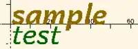
Supported font file formats are TrueType fonts (*.ttf) and OpenType fonts (*.otf). Once a file is registered to the project the details of the fonts in it may be seen in the font list dialog (see image) so that the logical font names, variations, and their available styles are available for use in the project.
3D Text by Extrusion
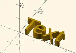
Text can be changed from a 2 dimensional object into a 3D object by using the linear_extrude function.
//3d Text Example
linear_extrude(4)
    text("Text");
Metrics
[Note: Requires version Development snapshot]
textmetrics() Function
The textmetrics() function accepts the same parameters as text(), and returns an object describing how the text would be rendered.
The returned object has these members:
- position
- a vector [X,Y], the origin of the first glyph, thus the lower-left corner of the drawn text.
- size
- a vector [a,b], the size of the generated text.

measurements of a glyph - ascent
- positive float, the amount that the text extends above the baseline.
- descent
- negative float, the amount that the text extends below the baseline.
- offset
- a vector default [0, 0], the lower-left corner of the box containing the text, including inter-glyph spacing before the first glyph.
- advance
- a vector default [153.09, 0], amount of space to leave to any following text.
This example displays the text metrics for the default font used by OpenSCAD:
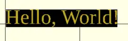
s = "Hello, World!";
size = 20;
font = "Liberation Serif";

tm = textmetrics(s, size=size, font=font);
echo(tm);
translate([0,0,1])
    text("Hello, World!", size=size, font=font);
color("black") translate(tm.position)
    square(tm.size); // "size" is of the bounding box
displays (formatted for readability):
ECHO: {
   position = [0.7936, -4.2752];
   size = [149.306, 23.552];
   ascent = 19.2768;
   descent = -4.2752;
   offset = [0, 0];
   advance = [153.09, 0];
   }
fontmetrics() Function
The fontmetrics() function accepts a font size and a font name, both optional, and returns an object describing global characteristics of the font.
Parameters
- size
- Decimal, optional. The size of the font, as described above for
text().
- font
- String, optional. The name of the font, as described above for
text().
Note that omitting the size and/or font may be useful to get information about the default font.
Returns an object:
- nominal: usual dimensions for a glyph:
- ascent: height above the baseline
- descent: depth below the baseline
- max: maximum dimensions for a glyph:
- ascent: height above the baseline
- descent: depth below the baseline
- interline: design distance from one baseline to the next
- font: identification information about the font:
- family: the font family name
- style: the style (Regular, Italic, et cetera)
echo(fontmetrics(font="Liberation Serif"));
yields (reformatted for readability):
   ECHO: {
       nominal = {
           ascent = 12.3766;
           descent = -3.0043;
       };
       max = {
           ascent = 13.6312;
           descent = -4.2114;
       };
       interline = 15.9709;
       font = {
           family = "Liberation Serif";
           style = "Regular";
       };
   }
Extrusion is the process of creating an object with a fixed cross-sectional profile. OpenSCAD provides two commands to create 3D solids from a 2D shape: linear_extrude() and rotate_extrude().
Linear extrusion is similar to pushing clay through a die with a profile shape cut through it.
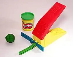
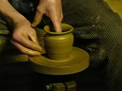
Rotational extrusion is similar to the process of applying a profile to clay spinning on a potter's wheel.
Both extrusion methods work on a (possibly disjointed) 2D shape normally drawn in the relevant plane (see below).
linear_extrude() Operator Module
A Linear Extrusion must be given a 2D child object, as in this statement:
linear_extrude( h=2 ) square();
This child object is first projected onto the X-Y plane along the Z axis to create the starting face of the extrusion. The start face is duplicated at the Z position given by the height parameter to create the extrusion's end face. The extrusion is then formed by creating a surface that joins each point along the edges of the two faces.
The 2D shape may be any 2D primitive shape, a 2d polygon, an imported 2D drawing, or a boolean combination of them. The 2D shape may have a Z value that moves it out of the X-Y plane, and it may even be rotated out of parallel with it. As stated above, the extrusion's starting face is the projection of the 2D shape onto the X-Y plane, which, if it is rotated, will have the effect of fore-shortening it normal to the axis of the rotation.
Using a 3D object as the extrusion's child will cause a compile time error. Including a 3D object in a composition of 2D objects (formed using boolean combinations on them) will be detected, the 3D object(s) will be deleted from it and the remaining 2D objects will be the basis for projecting their shape onto the X-Y plane.
Parameters For Linear Extrusion
There are no required parameters. The default operation is to extrude the child by 100 units vertically from the X-Y Plane, centered on the [0,0] origin.
- 1) height
- a non-negative integer, default 100, giving the length of the extrusion
- 2) v - twist axis vector
- a vector of 3 signed decimal values, default [0,0,1], used as an eigen vector specifying the axis of rotation for the twist. [Note: Requires version Development snapshot]
- 3) center
- a boolean, default false, that, when true, causes the resulting solid to be vertically centered at the X-Y plane.
- 4) convexity
- a non-negative integer, default 1, giving a measure of the complexity of the generated surface. See the Section on Convexity later on this page.
- 5) twist
- a signed decimal, default 0.0, specifying how many degrees of twist to apply between the start and end faces of the extrusion. 180 degrees is a half twist, 360 is all the way around, and so on.
- 6) scale
- either : a non-negative, decimal value, default 1.0, minimum 0.0, that specifies the factor by which the end face should be scaled up, or down, in size from that of the start face.
- or : an [x,y] vector that scales the extrusion in the X and Y directions separately.
- 7) slices
- a non-negative integer for the number of rows of polygons that the extr.
- 8) segments
- Similar to slices but adding points on the polygon's segments without changing the polygon's shape.
- h
- a named parameter, synonym to height
- $fn $fs $fa
- Special Parameters - given as named parameters.
Center
This parameter affects only affects the vertical position or the extrusion. Its X-Y position is always that of the projection that sets its starting face.
Scale
This is multiplicative factor that affects the size of extrusion's end face. As such 1.0 means no change, a value greater than one expands the end face, and a value between 0.001 and less than 1 shrinks it. A value of 0.0 causes the end face to degenerate to a point, turning the extrusion into a pyramid, cone, or complex pointy shape according to what the starting shape is.
Using the vector form sets the scale factor in the X and Y directions separately
Twist
Twist is applied, by default, as a rotation about the Z Axis. When the start face is at the origin a twist creates a spiral out of any corners in the child shape. If the start face is translated away from the origin the twist creates a spring shape.
A positive twist rotates clockwise, negative twist the opposite.
Twist Axis Vector
The second parameter is an [x,y,z] eigen vector that specifies the axis of rotation of the applied twist. The ratios of the three dimensional values to their respective coordinate axes specify the tilt away from the default axis, [0,0,1], the Z-Axis. For instance, v=[cos(45),0,1] tilts the extrusion at 45 degrees to the X axis.
The start and end faces are always normal to the Z-axis, even when the twist axis is tilted. The extruded and twisted surfaces are thus distorted from what might be expected in an extruded shape. The more expected result may be achieved by applying a rotation to then twisted extrusion on the Z Axis to tilt it into the desired position.
$fn, $fa, $fs Special Parameters
The special variables must be given as named parameters and are applied to the extrusion, overriding the global setting. When the same special variables are set on the base shape its values override their use as parameters on the extrusion.
Extrusion From Imported DXF
Example of linear extrusion of a 2D object imported from a DXF file.
linear_extrude(height = fanwidth, center = true, convexity = 10)
   import (file = "example009.dxf", layer = "fan_top");

A Unit Circle with No Twist
Generate an extrusion from a circle 2 units along the X Axis from the origin, centered vertically on the X-Y plane, with no twist. The extrusion appears to have a pentagonal cross-section because the extrusion's child is a 2D circle with the default value for $fn.
linear_extrude(height = 10, center = true, convexity = 10, twist = 0)
    translate([2, 0, 0])
        circle(r = 1);

A Unit Circle Twisted Left 100 Degrees
The same circle, but now with 100 degrees of counter-clockwise twist.
linear_extrude(height = 10, center = true, convexity = 10, twist = -100)
    translate([2, 0, 0])
        circle(r = 1);

A Unit Circle Twisted Right 100 Degrees
The same circle, but now with 100 degrees of clockwise twist.
linear_extrude(height = 10, center = true, convexity = 10, twist = 100)
    translate([2, 0, 0])
        circle(r = 1);

A Unit Circle Twisted Into a Spiral
The same circle, but made into a spiral by 500 degrees of counter-clockwise twist.
linear_extrude(height = 10, center = true, convexity = 10, twist = -500)
    translate([2, 0, 0])
        circle(r = 1);
Center
With center=false, the default, the extrusion is based on the X-Y plane and rises up in the positive Z direction.

When true it is centered vertically at the X-Y plane, as seen here:
Mesh Refinement
The slices parameter defines the number of intermediate points along the Z axis of the extrusion. Its default increases with the value of twist. Explicitly setting slices may improve the output refinement. Additional the segments parameter adds vertices (points) to the extruded polygon resulting in smoother twisted geometries. Segments need to be a multiple of the polygon's fragments to have an effect (6 or 9.. for a circle($fn=3), 8,12.. for a square() ).

linear_extrude(height = 10, center = false, convexity = 10, twist = 360, slices = 100)
translate([2, 0, 0])
circle(r = 1);
The special variables $fn, $fs and $fa can also be used to improve the output. If slices is not defined, its value is taken from the defined $fn value.

linear_extrude(height = 10, center = false, convexity = 10, twist = 360, $fn = 100)
translate([2, 0, 0])
circle(r = 1);
Scale
Scales the 2D shape by this value over the height of the extrusion. Scale can be a scalar or a vector:
 linear_extrude(height = 10, center = true, convexity = 10, scale=3)
 translate([2, 0, 0])
 circle(r = 1);

 linear_extrude(height = 10, center = true, convexity = 10, scale=[1,5], $fn=100)
 translate([2, 0, 0])
 circle(r = 1);

Note that if scale is a vector, the resulting side walls may be nonplanar. Use twist=0 and the slices parameter to avoid asymmetry.
 linear_extrude(height=10, scale=[1,0.1], slices=20, twist=0)
 polygon(points=[[0,0],[20,10],[20,-10]]);
Using with imported SVG
A common usage of this function is to import a 2D svg
 linear_extrude(height = 10, center = true)
 import("knight.svg");
rotate_extrude() Operator Module
Rotational extrusion spins a 2D shape around the Z-axis to form a solid which has rotational symmetry. One way to think of this operation is to imagine a Potter's wheel placed on the X-Y plane with its axis of rotation pointing up towards +Z. Then place the to-be-made object on this virtual Potter's wheel (possibly extending down below the X-Y plane towards -Z). The to-be-made object is the cross-section of the object on the X-Y plane (keeping only the right half, X >= 0). That is the 2D shape that will be fed to rotate_extrude() as the child in order to generate this solid. Note that the object started on the X-Y plane but is tilted up (rotated +90 degrees about the X-axis) to extrude.
Since a 2D shape is rendered by OpenSCAD on the X-Y plane, an alternative way to think of this operation is as follows: spins a 2D shape around the Y-axis to form a solid. The resultant solid is placed so that its axis of rotation lies along the Z-axis.
Just like the linear_extrude, the extrusion is always performed on the projection of the 2D polygon to the XY plane. Transformations like rotate, translate, etc. applied to the 2D polygon before extrusion modify the projection of the 2D polygon to the XY plane and therefore also modify the appearance of the final 3D object.
- A translation in Z of the 2D polygon has no effect on the result (as also the projection is not affected).
- A translation in X increases the diameter of the final object.
- A translation in Y results in a shift of the final object in Z direction.
- A rotation about the X or Y axis distorts the cross section of the final object, as also the projection to the XY plane is distorted.
Don't get confused, as OpenSCAD displays 2D polygons with a certain height in the Z direction, so the 2D object (with its height) appears to have a bigger projection to the XY plane. But for the projection to the XY plane and also for the later extrusion only the base polygon without height is used.
You cannot use rotate_extrude to produce a helix or screw thread. Doing this properly can be difficult, so it's best to find a thread library to make them for you.
The 2D shape must lie completely on either the right (recommended) or the left side of the Y-axis. More precisely speaking, every vertex of the shape must have either x >= 0 or x <= 0. If the shape spans the X axis a warning appears in the console windows and the rotate_extrude() is ignored. If the 2D shape touches the Y axis, i.e. at x=0, it must be a line that touches, not a point, as a point results in a zero thickness 3D object, which is invalid and results in a CGAL error. For OpenSCAD versions prior to 2016.xxxx, if the shape is in the negative axis the resulting faces are oriented inside-out, which may cause undesired effects.
Usage
rotate_extrude(angle = 360, start=0, convexity = 2) {...}

In 2021.01 and previous, you must use parameter names due to a backward compatibility issue.
- convexity : If the extrusion fails for a non-trival 2D shape, try setting the convexity parameter (the default is not 10, but 10 is a "good" value to try). See explanation further down.
- angle [Note: Requires version 2019.05] : Defaults to 360. Specifies the number of degrees to sweep, starting at the positive X axis. The direction of the sweep follows the Right Hand Rule, hence a negative angle sweeps clockwise.
- start [Note: Requires version Development snapshot] : Defaults to 0 if angle is specified, and 180 if not. Specifies the starting angle of the extrusion, counter-clockwise from the positive X axis.
- $fa : minimum angle (in degrees) of each fragment.
- $fs : minimum circumferential length of each fragment.
- $fn : fixed number of fragments in 360 degrees. Values of 3 or more override $fa and $fs
- $fa, $fs and $fn must be named parameters. click here for more details,.
Rotate Extrude on Imported DXF
rotate_extrude(convexity = 10)
   import (file = "example009.dxf", layer = "fan_side", origin = fan_side_center);
Examples
→
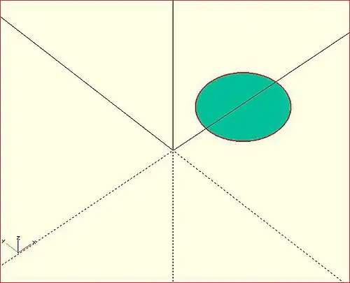
A simple torus can be constructed using a rotational extrude.
rotate_extrude(convexity = 10)
    translate([2, 0, 0])
        circle(r = 1);
Mesh Refinement
→
Increasing the number of fragments composing the 2D shape improves the quality of the mesh, but takes longer to render.
rotate_extrude(convexity = 10)
    translate([2, 0, 0])
        circle(r = 1, $fn = 100);
→
The number of fragments used by the extrusion can also be increased.
rotate_extrude(convexity = 10, $fn = 100)
    translate([2, 0, 0])
        circle(r = 1, $fn = 100);
Using the parameter angle (with OpenSCAD versions 2016.xx), a hook can be modeled .
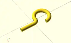
eps = 0.01;
translate([eps, 60, 0])
    rotate_extrude(angle=270, convexity=10)
        translate([40, 0]) circle(10);
rotate_extrude(angle=90, convexity=10)
    translate([20, 0]) circle(10);
translate([20, eps, 0])
    rotate([90, 0, 0]) cylinder(r=10, h=80+eps);
Extruding a Polygon
Extrusion can also be performed on polygons with points chosen by the user.
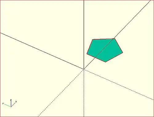
Here is a simple polygon and its 200 step rotational extrusion. (Note it has been rotated 90 degrees to show how the rotation appears; the rotate_extrude() needs it flat).
rotate([90,0,0]) polygon( points=[[0,0],[2,1],[1,2],[1,3],[3,4],[0,5]] );
rotate_extrude($fn=200) polygon( points=[[0,0],[2,1],[1,2],[1,3],[3,4],[0,5]] );
→ →
→
For more information on polygons, please see: 2D Primitives: Polygon.
Orientation
If you're making a round 360 degree extrusion, it doesn't matter where it starts. If, on the other hand, you're using $fn to make an extrusion with some specific number of sides, it can matter. With an odd number of sides, there will be a vertex on either the left or the right, and a side opposite it.
With angle not specified, the extrusion starts along the negative X axis, to the left of the origin. With an odd number of sides, there is a vertex on the left and a side on the right. (Note that this is inconsistent with the behavior for angle less than 360, and with the behavior for circle and other round primitives.)
With angle specified, and not equal to 360, the extrusion starts along the positive X axis, to the right of the origin.
For 2021.01 and earlier, if angle is equal to 360, the extrusion starts along the negative X axis, as for angle not being specified.
For the development snapshot, if angle is 360, the extrusion starts along the positive X axis, as for other cases where angle is specified. Explicitly specifying angle=360 thus yields results consistent with other round primitives.
A future release may change this behavior so that when angle is not specified the extrusion starts along the positive X axis, making all of these cases consistent.
start directly controls the start point. [Note: Requires version Development snapshot]
Description of extrude parameters
Parameters Used In All Extrusions
- convexity
- an integer that works as a measure of complexity based on the maximum number of sides a ray might penetrate as it passes through a shape.
For instance, the convexity of a sphere is one and the convexity of a torus is two. From any point of view there is only a single surface showing for a sphere. But with a torus a given pixel may be showing the front most face, the back part of the doughnut, or the background. Setting convexity greater than the default 1 informs the renderer of the need to be more careful in its work.
Arbitrarily setting convexity to 10 should solve most preview rendering issues, at the expense of slowing preview rendering. When a model has several convoluted shapes values more than 15 can slow rendering to the point of freezing the application.
The issue of Convexity is an issue in Preview Rendering.
Parameters For Linear Extrusion
- height
- a non-negative integer, default 100, giving the length of the extrusion
- center
- a boolean, default false, that, when true, causes the resulting solid to be vertically centered at the X-Y plane.
- twist
- a signed decimal, default 0.0, specifying how many degrees of twist to apply between the start and end faces of the extrusion
- scale
- a non-negative, decimal value, default 1.0, greater than 0.0, that specifies the factor by which the end face should be scaled up, or down, in size from that of the start face.
- a vector containing these values in this order
- [
- slices
- a non-negative integer value that acts on the extruded surface as $fn does, but which is not applied to the child 2D shape.
- segments
- Similar to slices but adding points on the polygon's segments without changing the polygon's shape.
- $fn
- the special variable but applied only to the extrusion
- $fs
- the special variable but applied only to the extrusion
- $fa
- the special variable but applied only to the extrusion
- ]
Note
- centering the extrusion only affects its vertical position. Its X-Y position is always set by its starting face.
- A Scale Factor greater than one increases the size of the extrusion's end face, while a value greater than 0.0 and less than 1 shrink it. A value of 0.0 causes the end face to degenerate to a point, turning the extrusion into a pyramid, cone, or complex pointy shape according to what the starting shape is.
Chapter 4 -- Transform
OpenSCAD User Manual/The OpenSCAD Language
Transforms Affect Nodes
Transformations are applied to modify position, orientation, or size by writing them at the beginning of a line of OpenSCAD code that defines a new node. Nodes are defined as primitive shapes or CSG Modelling Operations or looping and conditional statements that form syntactic groups.
The simplest form for statements that define shapes is
<transform>*<child node>;
meaning that zero or more (shown by *) calls to transform modules can precede code that defines a node. The node thus created may be as simple as a single shape, or may be a complex of nested language elements that define an assembly of shapes, but in all cases the combined effect of the transforms are applied to the single child node that must be the last item on the line. Indentation is commonly used to make the child nodes more visible for the reader, but as this example shows, these two statements are identical.
translate([10,20,30]) cube(10);
translate([10,20,30])
    cube(10);
In the OpenSCAD language semicolons mark the end of a line of code so if one is placed after a transform module call it means there will be no child node created.
Transform modules can be applied to grouped statements using braces ( '{ }' to enclose the sub-tree in this manner:
translate([0,0,-5])
    {
    cube(10);
    cylinder(r=5,h=10);
    }
translate([0,0,-5]) { cube(10); cylinder(r=5,h=10); }
Like the previous code example the two statements are identical in meaning but indentation makes the first more readable. Also note that a statement group is not ended by a semi-colon, but each separate line in the group but be ended by one, including the last.
Indentation is commonly used to show the scope of transform module calls but they are always applied outwards from the child object, not in the sequence written in the statement.
rotate([45,45,45])
    translate([10,20,30])
        cube(10);
Syntactic Order Versus Mathematical
The order of calls to transform modules makes no difference to the correctness of a statement syntactically, but for some the order of operations is significant. A call to set the colour of an object may be inserted anywhere, but those that affect the child geometry have to be correctly ordered.
color("red")     translate([0,10,0])  rotate([45,0,0]) cube(5);
rotate([45,0,0]) translate([0,10,0])  color("green")   cube(5);
Both translation and rotation module calls are the same, but moving the second cube and then rotating it, is not the same as first rotating the first cube, then moving it away from the origin. In the second case the rotation causes the cube to move along an arc 10 units from the origin, the first the cube is rotated them moved along the Y axis.
Differences in Preview Rendering
OpenSCAD uses a different library to preview simple transforms (translate, rotate, etc.) than for more advanced transforms, like resize. The effects of modifier characters, specifically "#" and "%", on the rendered objects may not match expectations. A shape with only simple transforms applied will be rendered in its post-transformation form, while the highlight for a resized shape will be applied to its original form.
Transform Modules
Scale
Scales its child elements using the specified vector. Using the name of the argument is optional.
Usage Example:
scale(v = [x, y, z]) { ... }
cube(10);
translate([15,0,0]) scale([0.5,1,2]) cube(10);
_example.JPG)
Resize
This module actually changes the form of the child node by the amount given by the x,y, and z dimensions of the given vector. If an amount is zero that dimension is not changed
resize() is an operation from the CGAL library and as such operates on the full geometry of the child node and its use can make for longer rendering time in preview mode.
Usage Example:
// resize the sphere to extend 30 in x, 60 in y, and 10 in the z directions.
resize(newsize=[30,60,10]) sphere(r=10);

// resize the 1x1x1 cube to 2x2x1
resize([2,2,0]) cube();
If the 'auto' parameter is set to true, it auto-scales any 0-dimensions to match. For example.
// resize the 1x2x0.5 cube to 7x14x3.5
resize([7,0,0], auto=true) cube([1,2,0.5]);
The 'auto' parameter can also be used if you only wish to auto-scale a single dimension, and leave the other as-is.
// resize to 10x8x1. Note that the z dimension is left alone.
resize([10,0,0], auto=[true,true,false]) cube([5,4,1]);
Scale vs Resize
In many cases the effect of scale() will be the same as for resize(), but when the child to be modified is not a symmetrical shape the effects can be seen to be different.
This image shows a default cube and a cube([3,2,5]) in white, both transformed by resize([2,2,0]) and then scaled by scale([2,2,1]). The scale.z value must be 1 to preserve the cube's Z dimension.
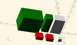
The resize operation on the cube([3,2,5]) shortens it to match the [2,2,0] size while the scale just makes it bigger in all dimensions.
Rotate
This module acts to rotate its children through a given angle about an axis. The angle and the axis may be given in different forms to facilitate programming needs. The argument names are optional when values are given in the order of the following specification.
The angle of rotation must be given in degrees and may be a decimal fraction. In its simplest form the effect is to rotate the child around the Z-axis by the given value, "angle", in degrees. This is useful in 2D contexts where that is the only axis for rotation.
rotate( <angle> );
The angle may also be given as a named parameter "a", thus: rotate( a=<angle> ).
For example:
rotate(45) square(10);

as seen in this image
An optional argument, "v", may be given to define the axis about which the child is rotated. It its simplest form just one of the X, Y, or Z elements will have value one (1) to specify the single coordinate axis will be the basis for rotation. For example to rotate 180 degrees around the Y-axis we can use:
rotate(a=180, v=[0,1,0]) { ... }
The "v=[x,y,z]" parameter is as a Euler vector that can define any arbitrary axis for rotation. The three components may be given as signed, decimal float values that define a line in 3-space around which the child node will be rotated. This does not give the same result as using the a=[x_rot,y_rot,z_rot] form shown in a following section, but has the same mathematical basis.
For example using the "v" form to rotate a child node by 45 degrees around an axis halfway between the X and Y coordinate axes uses the vector [1,1,0] as in this code:
rotate(a=45, v=[1,1,0]) { ... }
giving this result:
_example.JPG)
In its full form the module call has this form:
rotate(a = deg_a, v = [x, y, z]) // named parameters
rotate( a, [x, y, z] ) // positional parameters

rotate( 30, [.5,.5,.5] )
    cube([2,4,6]);
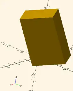
Combination of Three Rotations
Alternately the angle of rotation may be given as a vector of angles:
rotate(a = [x_rot, y_rot, z_rot]) // named parameter "a"
rotate([deg_x, deg_y, deg_z])     // positional parameters
In this form the axis argument ("v") is ignored. The three angular rotations are applied in order of x_rot first, then y_rot, and finally z_rot. The following code fragment is a reminder that the transform "closest" to the child node is the operation carried out first.
rotate(a=[0,0,az])
    rotate(a=[0,ay,0])
        rotate(a=[ax,0,0])
            { <child node> }
Rotate vs Mirror
It is worth noting that while in some cases rotating an object by 180 degrees around an axis results in the same geometry as mirroring it in a suitable plane, mathematically these are different operations that create unique geometries, as the following code will illustrate:
transf = true; // [true,false]

mirr = transf ? 1 : 0;
rotat = transf ? 180 : 0;

mirror([0,0,mirr])
union(){
    color("yellow", alpha=.30)
    cube( [5,8,2],center=true );
    translate( [-1,0,-2] )
        color("red")
        cube( [3,3,5] );
    translate( [0,-5,-2] )
        color("green")
        cube( [3,3,5] );
    }

translate( [-10,0,0] )
    rotate([rotat,0,0])
union(){
    color("yellow", alpha=.30)
    cube( [5,8,2],center=true );
    translate( [-1,0,-2] )
        color("red")
        cube( [3,3,5] );
    translate( [0,-5,-2] )
        color("green")
        cube( [3,3,5] );
    }
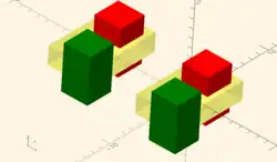
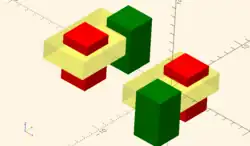
Rotation rule help
For the case of:
rotate([a, b, c]) { ... };
"a" is a rotation about the X axis, from the +Y axis, toward the +Z axis.
"b" is a rotation about the Y axis, from the +Z axis, toward the +X axis.
"c" is a rotation about the Z axis, from the +X axis, toward the +Y axis.
These are all cases of the Right Hand Rule. Point your right thumb along the positive axis, your fingers show the direction of rotation.
Thus if "a" is fixed to zero, and "b" and "c" are manipulated appropriately, this is the spherical coordinate system.
So, to construct a cylinder from the origin to some other point (x,y,z):
x= 10; y = 10; z = 10; // point coordinates of end of cylinder

length = norm([x,y,z]);  // radial distance
b = acos(z/length); // inclination angle
c = atan2(y,x);     // azimuthal angle

rotate([0, b, c])
    cylinder(h=length, r=0.5);
%cube([x,y,z]); // corner of cube should coincide with end of cylinder

Translate
Translate moves its child node for the distances given in the three elements of the given vector. The argument name, "v", is optional.
Example:
translate(v = [x, y, z]) { ... }
In the following code there is a cube of 2 units square centered on the origin with no transform applied, with a unit sphere as a child node of a X=5 units translation.
cube(2,center = true);
translate([5,0,0])
   sphere(1,center = true);
_example.JPG)
Mirror
The effect of this transform is to project the geometry of its child node through a mirror plane to the equidistant position on the plane's other side. Mirrors are planes that pass through the origin with the orientation given by its Normal Vector. This specific normal vector is given as the "v=[x,y,z]" parameter to mirror() which is is a Euler vector with values being signed, decimal floats.
In its simplest form just one of the elements will have a non-zero value. So to mirror something in the Y-Z plane the vector is the X-axis ( v=[1,0,0] ). Note that a Euler vector takes the ratios between its components for its direction, not the absolute values. Thus the proportions of v=[1,0,0], v=[-1,0,0], v=[0.05,0,0], and v=[100,0,0] all describe the same vector, the X-axis.
In general the signs of the vector elements are significant, so for instance the planes for v=[1,1,0] and v=[1,-1,0] are at right angles to each other. But the lines for v=[1,1,0] and v=[-1,-1,0] are the same line, just in opposite directions.
The operation of the transform is to project each point of the child node to the mirror plane along a line drawn normal to the plane. Each point is then projected through the mirror for the same distance on the other side to create the mirrored child node.
For example, for a cube entirely in the positive X half of the modelling space applying mirror([1,0,0]), changes the x coordinate of its every point from positive to negative.
It is worth pointing out that mirror() "moves" the child node, it does not make a new copy of it.
Function signature:
mirror(v= [x, y, z] ) { ... }
Examples
The original is on the right hand side.
-
![hand(); // original mirror([1,0,0]) hand();](../_assets_/0c70a452f799bfe840676ee341124611/Mirror-x.png)
hand(); // originalmirror([1,0,0]) hand(); -
![hand(); // original mirror([1,1,0]) hand();](../_assets_/0c70a452f799bfe840676ee341124611/Mirror-x-y.png)
hand(); // originalmirror([1,1,0]) hand(); -
![hand(); // original mirror([1,1,1]) hand();](../_assets_/0c70a452f799bfe840676ee341124611/Mirror-x-y-z.png)
hand(); // originalmirror([1,1,1]) hand();
 // original
 rotate([0,0,-30]){
   cube([23,12,10]);
   translate([0.5, 4.4, 9.9]){
     color("red", 1.0){
       linear_extrude(height=2){
         text("OpenSCAD", size= 3);
       }
     }
   }
 }
 // mirrored
 mirror([1,0,0]){
   rotate([0,0,-30]){
     cube([23,12,10]);
     translate([0.5, 4.4, 9.9]){
       color("red", 1.0){
         linear_extrude(height=2){
           text("OpenSCAD", size= 3);
         }
       }
     }
   }
 }

Multmatrix
Multiplies the geometry of all child elements with the given affine transformation matrix, where the matrix is 4×3 - a vector of 3 row vectors with 4 elements each, or a 4×4 matrix with the 4th row always forced to [0,0,0,1].
Usage: multmatrix(m = [...]) { ... }
This is a breakdown of what you can do with the independent elements in the matrix (for the first three rows):
| Scale X | Shear X along Y | Shear X along Z | Translate X |
| Shear Y along X | Scale Y | Shear Y along Z | Translate Y |
| Shear Z along X | Shear Z along Y | Scale Z | Translate Z |
The fourth row is forced to [0,0,0,1] and can be omitted unless you are combining matrices before passing to multmatrix, as it is not processed in OpenSCAD. Each matrix operates on the points of the given geometry as if each vertex is a 4 element vector consisting of a 3D vector with an implicit 1 as its 4th element, such as v=[x, y, z, 1]. The role of the implicit fourth row of m is to preserve the implicit 1 in the 4th element of the vectors, permitting the translations to work. The operation of multmatrix therefore performs m*v for each vertex v. Any elements (other than the 4th row) not specified in m are treated as zeros.
This example rotates by 45 degrees in the XY plane and translates by [10,20,30], i.e. the same as translate([10,20,30]) rotate([0,0,45]) would do.
angle=45;
multmatrix(m = [ [cos(angle), -sin(angle), 0, 10],
                 [sin(angle),  cos(angle), 0, 20],
                 [         0,           0, 1, 30],
                 [         0,           0, 0,  1]
              ]) union() {
   cylinder(r=10.0,h=10,center=false);
   cube(size=[10,10,10],center=false);
}
The following example demonstrates combining affine transformation matrices by matrix multiplication, producing in the final version a transformation equivalent to rotate([0, -35, 0]) translate([40, 0, 0]) Obj();. Note that the signs on the sin function appear to be in a different order than the above example, because the positive one must be ordered as x into y, y into z, z into x for the rotation angles to correspond to rotation about the other axis in a right-handed coordinate system.
module Obj() {
   cylinder(r=10.0,h=10,center=false);
   cube(size=[10,10,10],center=false);
}

// This itterates into the future 6 times and demonstrates how multimatrix is moving the object around the center point
for(time = [0 : 15 : 90]){
    y_ang=-time;
    mrot_y = [ [ cos(y_ang), 0,  sin(y_ang), 0],
               [         0,  1,           0, 0],
               [-sin(y_ang), 0,  cos(y_ang), 0],
               [         0,  0,           0, 1]
             ];
    mtrans_x = [ [1, 0, 0, 40],
                 [0, 1, 0,  0],
                 [0, 0, 1,  0],
                 [0, 0, 0,  1]
               ];

    echo(mrot_y*mtrans_x);

    // This is the object at [0,0,0]
    Obj();

    // This is the starting object at the [40,0,0] coordinate
    multmatrix(mtrans_x) Obj();

    // This is the one rotating and appears 6 times
    multmatrix(mrot_y * mtrans_x) Obj();
};
This example skews a model, which is not possible with the other transformations.
M = [ [ 1  , 0  , 0  , 0   ],
      [ 0  , 1  , 0.7, 0   ],  // The "0.7" is the skew value; pushed along the y axis as z changes.
      [ 0  , 0  , 1  , 0   ],
      [ 0  , 0  , 0  , 1   ] ] ;
multmatrix(M) {  union() {
    cylinder(r=10.0,h=10,center=false);
    cube(size=[10,10,10],center=false);
} }
This example shows how a vector is transformed with a multmatrix vector, like this all points in a point array (polygon) can be transformed sequentially. Vector (v) is transformed with a rotation matrix (m), resulting in a new vector (vtrans) which is now rotated and is moving the cube along a circular path radius=v around the z axis without rotating the cube.
angle=45;
 m=[
        [cos(angle), -sin(angle), 0, 0],
        [sin(angle),  cos(angle), 0, 0],
        [         0,           0, 1, 0]
   ];

v=[10,0,0];
vm=concat(v,[1]); // need to add [1]
vtrans=m*vm;
echo(vtrans);
translate(vtrans)cube();
More?
Learn more about it here:
Color
Displays the child elements using the specified RGB color + alpha value. This is only used for the F5 preview as CGAL and STL (F6) do not currently support color. The alpha value defaults to 1.0 (opaque) if not specified.
Function Form
color( c = [r, g, b, a] ) { ... }
color( c = [r, g, b], alpha = 1.0 ) { ... }
color( "#hexvalue" ) { ... }
color( "colorname", 1.0 ) { ... }
Note that the r, g, b, a values are limited to floating point values in the range [0,1] rather than the more traditional integers { 0 ... 255 }. However, nothing prevents you from using R, G, B values from {0 ... 255} with appropriate scaling: color([ R/255, G/255, B/255 ]) { ... }
[Note: Requires version 2011.12]
Colors can also be defined by name (case insensitive). For example, to create a red sphere, you can write color("red") sphere(5);. Alpha is specified as an extra parameter for named colors: color("Blue",0.5) cube(5);
[Note: Requires version 2019.05]
Hex values can be given in 4 formats, #rgb, #rgba, #rrggbb and #rrggbbaa. If the alpha value is given in both the hex value and as separate alpha parameter, the alpha parameter takes precedence.
Warning: alpha channel processing (transparency) is order-sensitive. Transparent objects must be listed after non-transparent objects to display them correctly. Some combinations involving multiple transparent objects cannot be handled correctly. See issue #1390.
The available color names are taken from the World Wide Web consortium's SVG color list. A chart of the color names is as follows,
(note that both spellings of grey/gray including slategrey/slategray etc are valid):
|
|
|
|
| |||||||||||||||||||||||||||||||||||||||||||||||||||||||||||||||||||||||||||||||||||||||||||||||||||||||||||||||||||||||||||||||||||||||||||||||||||||||||
Example
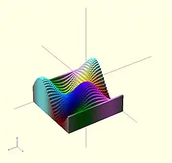
Here's a code fragment that draws a wavy multicolor object
  for(i=[0:36]) {
    for(j=[0:36]) {
      color( [0.5+sin(10*i)/2, 0.5+sin(10*j)/2, 0.5+sin(10*(i+j))/2] )
      translate( [i, j, 0] )
      cube( size = [1, 1, 11+10*cos(10*i)*sin(10*j)] );
    }
  }
↗ Being that -1<=sin(x)<=1 then 0<=(1/2 + sin(x)/2)<=1 , allowing for the RGB components assigned to color to remain within the [0,1] interval.
Chart based on "Web Colors" from Wikipedia
Example 2
In cases where you want to optionally set a color based on a parameter you can use the following trick:
 module myModule(withColors=false) {
    c=withColors?"red":undef;
    color(c) circle(r=10);
 }
Setting the colorname to undef keeps the default colors.
Offset
[Note: Requires version 2015.03]
Offset generates a new 2d interior or exterior outline from an existing outline. There are two modes of operation: radial and delta.
- The radial method creates a new outline as if a circle of some radius is rotated around the exterior (r > 0) or interior (r < 0) of the original outline.
- The delta method creates a new outline with sides having a fixed distance outward (delta > 0) or inward (delta < 0) from the original outline.
The construction methods produce an outline that is either inside or outside of the original outline. For outlines using delta, when the outline goes around a corner, it can be given an optional chamfer.
Offset is useful for making thin walls by subtracting a negative-offset construction from the original, or the original from a positive offset construction.
Offset can be used to simulate some common solid modeling operations:
- Fillet:
offset(r=-3) offset(delta=+3)rounds all inside (concave) corners, and leaves flat walls unchanged. However, holes less than 2*r in diameter vanish. - Round:
offset(r=+3) offset(delta=-3)rounds all outside (convex) corners, and leaves flat walls unchanged. However, walls less than 2*r thick vanish.
- Parameters
The first parameter may be passed without a name, in which case it is treated as the r parameter below. All other parameters must be named if used.
r or delta
- Number. Amount to offset the polygon. When negative, the polygon is offset inward.
- r (default parameter if not named) specifies the radius of the circle that is rotated about the outline, either inside or outside. This mode produces rounded corners. The name may be omitted; that is,
offset(c)is equivalent tooffset(r=c). - delta specifies the distance of the new outline from the original outline, and therefore reproduces angled corners. No inward perimeter is generated in places where the perimeter would cross itself.
- r (default parameter if not named) specifies the radius of the circle that is rotated about the outline, either inside or outside. This mode produces rounded corners. The name may be omitted; that is,
- chamfer
- Boolean. (default false) When using the delta parameter, this flag defines if edges should be chamfered (cut off with a straight line) or not (extended to their intersection). This parameter has no effect on radial offsets.
$fa, $fs, and $fn
- The circle resolution special variables may be used to control the smoothness or facet size of curves generated by radial offsets. They have no effect on delta offsets.
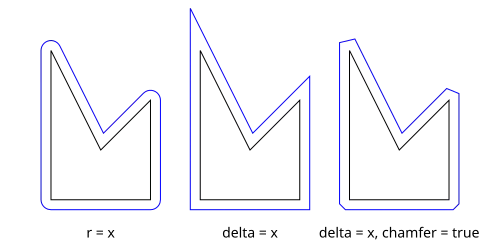
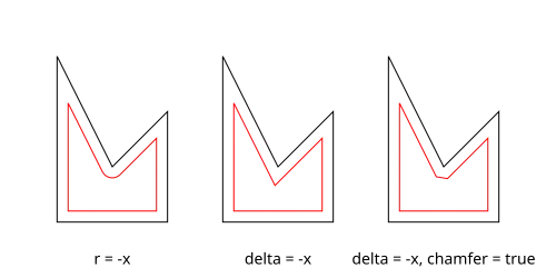
Examples
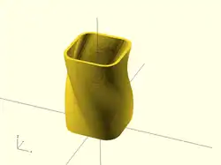
// Example 1

linear_extrude(height = 60, twist = 90, slices = 60) {
   difference() {
     offset(r = 10) {
      square(20, center = true);
     }
     offset(r = 8) {
       square(20, center = true);
     }
   }
 }
// Example 2

module fillet(r) {
   offset(r = -r) {
     offset(delta = r) {
       children();
     }
   }
}
Fill
[Note: Requires version Development snapshot]
The fill() operation removes holes from polygons without changing the outline. For convex polygons the result is identical to hull().
Examples
// Example 1

t = "OpenSCAD";

linear_extrude(15) {
	text(t, 50);
}
color("darkslategray") {
	linear_extrude(2) {
		offset(4) {
			fill() {
				text(t, 50);
			}
		}
	}
}
Minkowski
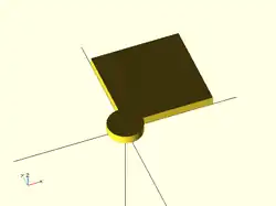
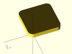
Displays the minkowski sum of child nodes.
Usage example:
Say you have a flat box, and you want a rounded edge. There are multiple ways to do this (for example, see hull below), but minkowski is elegant. Take your box, and a cylinder:
 $fn=50;
 cube([10,10,1]);
 cylinder(r=2,h=1);
Then, do a minkowski sum of them (note that the outer dimensions of the box are now 10+2+2 = 14 units by 14 units by 2 units high as the heights of the objects are summed):
$fn=50;
minkowski()
{
  cube([10,10,1]);
  cylinder(r=2,h=1);
}
NB: The origin of the second object is used for the addition. The following minkowski sums are different: the first expands the original cube by +1 in -x, +x, -y, +y from cylinder, expand 0.5 units in both -z, +z from cylinder. The second expands it by +1 in -x, +x, -y, +y and +z from cylinder, but expand 0 in the -z from cylinder.
minkowski() {
	cube([10, 10, 1]);
	cylinder(1, center=true);
}
minkowski() {
	cube([10, 10, 1]);
	cylinder(1);
}
Warning: for high values of $fn the minkowski sum may end up consuming lots of CPU and memory, since it has to combine every child node of each element with all the nodes of each other element. So if for example $fn=100 and you combine two cylinders, then it does not just perform 200 operations as with two independent cylinders, but 100*100 = 10000 operations.
Warning: if one of the inputs is compound, such as:
    {
         translate([0, 0, collar])
         sphere(ball);
         cylinder(collar, ball, ball);
    }
it may be treated as two separate inputs, resulting in an output which is too large, and has features between surfaces that should be unaltered with respect to one another. If so, use union().
Hull
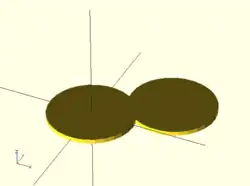
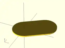
Displays the convex hull of child nodes.
Usage example:
hull() {
    translate([15,10,0]) circle(10);
    circle(10);
}
The Hull of 2D objects uses their projections (shadows) on the xy plane, and produces a result on the xy plane. Their Z-height is not used in the operation.
Referring to the illustration of a convex hull of two cylinders, it is computationally more efficient to use hull() on two 2D circles and linear_extrude the resulting 2D shape into a 3D shape, rather than using hull() on two cylinders, even though the resulting object appears identical. Complex geometries involving hull() can be rendered faster by starting out in 2D, if possible.
Chapter 5 -- Boolean combination
OpenSCAD User Manual/The OpenSCAD Language
boolean overview
2D examples
-
 union ( or )
circle + square -
 difference ( and not )
square - circle -
 difference ( and not )
circle - square -
 intersection ( and )
circle - (circle - square)
 union()       {square(10);circle(10);} // square or  circle
 difference()  {square(10);circle(10);} // square and not circle
 difference()  {circle(10);square(10);} // circle and not square
 intersection(){square(10);circle(10);} // square and circle
3D examples
-
 union ( or )
sphere + cube -
 difference ( and not )
cube - sphere -
 difference ( and not )
sphere - cube -
 intersection ( and )
sphere - (sphere - cube)
 union()       {cube(12, center=true); sphere(8);} // cube or  sphere
 difference()  {cube(12, center=true); sphere(8);} // cube and not sphere
 difference()  {sphere(8); cube(12, center=true);} // sphere and not cube
 intersection(){cube(12, center=true); sphere(8);} // cube and sphere
Union Operator Module
Creates a union of all its child nodes. This is the sum of all children (logical or).
May be used with either 2D or 3D objects, but don't mix them.

 //Usage example:
 union() {
 	cylinder (h = 4, r=1, center = true, $fn=100);
 	rotate ([90,0,0]) cylinder (h = 4, r=0.9, center = true, $fn=100);
 }
Remark: union is implicit when not used. But it is mandatory, for example, in difference to group first child nodes into one.
Note: It is mandatory for all unions, explicit or implicit, that external faces to be merged not be coincident. Failure to follow this rule results in a design with undefined behavior, and can result in a render which is not manifold (with zero volume portions, or portions inside out), which typically leads to a warning and sometimes removal of a portion of the design from the rendered output. (This can also result in flickering effects during the preview.) This requirement is not a bug, but an intrinsic property of floating point comparisons and the fundamental inability to exactly represent irrational numbers such as those resulting from most rotations. As an example, this is an invalid OpenSCAD program, and will at least lead to a warning on most platforms:
 // Invalid!
 size = 10;
 rotation = 17;
 union() {
    rotate([rotation, 0, 0])
       cube(size);
    rotate([rotation, 0, 0])
       translate([0, 0, size])
       cube([2, 3, 4]);
 }
The solution is to always use a small value called an epsilon when merging adjacent faces like this to guarantee overlap. Note the 0.01 eps value used in TWO locations, so that the external result is equivalent to what was intended:
 // Correct!
 size = 10;
 rotation = 17;
 eps = 0.01;
 union() {
    rotate([rotation, 0, 0])
       cube(size);
    rotate([rotation, 0, 0])
       translate([0, 0, size-eps])
       cube([2, 3, 4+eps]);
 }
Difference Operator Module
This operator does nothing when given a single child:
difference() cube();
Having it operate on two or more children performs the logical And-Not operation by deleting the shapes following the first from it.
Intersection may be applied to 2D or 3D objects, but should be applied to objects of only one type. Mixing 2D and 3D child nodes will give indeterminate results, if any.

Usage example:
difference() {
	cylinder (h = 4, r=1, center = true, $fn=100);
	rotate ([90,0,0]) cylinder (h = 4, r=0.9, center = true, $fn=100);
}
Note: It is mandatory that surfaces that are to be removed by a difference operation have an overlap, and that the negative piece being removed extends fully outside of the volume it is removing that surface from. Failure to follow this rule can cause preview artifacts and can result in non-manifold render warnings or the removal of pieces from the render output. See the description above in union for why this is required and an example of how to do this by this using a small epsilon value.
Difference With Multiple Children
Note, in the second instance, the result of adding a union of the 1st and 2nd children.

// Usage example for difference of multiple children:
$fn=90;
difference(){
    cylinder(r=5,h=20,center=true);
    rotate([00,140,-45])
        color("LightBlue")
            cylinder(r=2,h=25,center=true);
    rotate([00,40,-50])
        cylinder(r=2,h=30,center=true);
    translate([0,0,-10])
        rotate([00,40,-50])
            cylinder(r=1.4,h=30,center=true);
}

// second instance with added union
translate([10,10,0]){
    difference(){
      union(){        // combine 1st and 2nd children
                                                cylinder(r=5,h=20,center=true);
        rotate([00,140,-45]) color("LightBlue") cylinder(r=2,h=25,center=true);
      }
      rotate([00,40,-50])                       cylinder(r=2,h=30,center=true);
      translate([0,0,-10])rotate([00,40,-50])   cylinder(r=1.4,h=30,center=true);
    }
}
Intersection Operator Module
Creates the intersection of its child nodes. This logical and operation creates an object that is the overlapping part of all the child nodes together
Intersection may be applied to 2D or 3D objects, but should be applied to objects of only one type. Mixing 2D and 3D child nodes will give indeterminate results, if any.

//Usage example:
intersection() {
	cylinder (h = 4, r=1, center = true, $fn=100);
	rotate ([90,0,0])
        cylinder (h = 4, r=0.9, center = true, $fn=100);
    }
Chapter 6 -- Other Functions and Operators
OpenSCAD User Manual/The OpenSCAD Language
Conditional and Iterator Functions
For() Module
A module that will invoke its child module(s) repeatedly.
Format
for( <loop_var> ) <child expression>;
As with any module, the child of a for() may be a block of code in braces:
for( <loop_var> ) { one(); two(); x=12 };
Parameters
- <loop_vars>
- the loop variable determines how many times the <child expression> will be invoked. It is also a local variable in the scope of the <child expression>.
- <child expression>
- the loop will invoke this expression once for each value of the loop variable. It may be a statement, module call, or a block of statements in braces.
Loop Variable Formats
A for() loop must operate a fixed number of times as set by the loop variable. There are a number of formats for specifying the value that the loop variable will have in each iteration.
- Range
- for( r=[start:incr:end] ), 'r' will be a number in the sequence of the range.
for( r= [start : end] ) - Vector
- for( v = [vector] ), 'v' will be elements of the vector and so may be of any data type, or an unnamed function (a lambda function).
- String
- for( s = "string" ), 's' will be a single letter string
- Object
- for( o = object ), 'o' will be a string containing the name of a member of the object, in the order members were defined in.
Note: Loop variables for an object are only indirect references to the content of its members, unlike the other types. To access the members of an object the String-Index form may be used, member=object[o]
Range Examples
The normal way to use a range:
for (a =[3:5])echo(a); // 3 4 5
Counting down using a range [Deprecated: start > end is deprecated after 2015.03 and will be removedin a future release. Use negative increment instead]
 for (a =[3:0]){echo(a);}   // 0 1 2 3
 for (a =[3:-1:0]){echo(a);} // negative increment : 0 1 2 3
Note: The End must be less than start when increment is less than zero
Counting by fractions
for (a =[3.0 :0.5: 5.0])echo(a); // 3 3.5 4 4.5 5
Loop will stop when current_value + Increment > end so the end value may not be reached
for (a =[0:2:5])echo(a); // 0 2 4 : a + 2 > 4 stops the loop
Vector Examples
The loop value is defined with each element of the vector in order:
for (a =[3,4,1,5]) echo(a); // 3 4 1 5
It will be whatever data type the element is
for (a =[[1,2],6,"s",[[3,4],[5,6]]]) echo(a); // [1,2] 6 "s" [[3,4],[5,6]]
Object Examples
[Note: Requires version Development snapshot]
The loop value is defined with the name of each member of the object, in the order they were defined in.
thing = object( this="str", that=12 );
for( o=thing ) echo( o, thing[o] );
shows:
ECHO: "this", "str"
ECHO: "that", 12
There are built-in functions that return objects:
tm = textmetrics("Hello, World!");
for (name = tm) echo(name, tm[name]);
For is a Module
The for() is a module that invokes its child module repeatedly. The loop variable(s) are local to the scope of the for() and are defined separately in each branch of a tree of instances.
Hence:
for (i=[0:3])
   translate([i*10,0,0])
     cube(i+1);
Using menu Design > Display-CSG-Tree shows how the loop is unrolled and the variables are given fixed values in each instance:
group() {
    multmatrix([[1, 0, 0, 0], [0, 1, 0, 0], [0, 0, 1, 0], [0, 0, 0, 1]]) {
        cube(size = [1, 1, 1], center = false);
    }
    multmatrix([[1, 0, 0, 10], [0, 1, 0, 0], [0, 0, 1, 0], [0, 0, 0, 1]]) {
        cube(size = [2, 2, 2], center = false);
    }
    multmatrix([[1, 0, 0, 20], [0, 1, 0, 0], [0, 0, 1, 0], [0, 0, 0, 1]]) {
        cube(size = [3, 3, 3], center = false);
    }
    multmatrix([[1, 0, 0, 30], [0, 1, 0, 0], [0, 0, 1, 0], [0, 0, 0, 1]]) {
        cube(size = [4, 4, 4], center = false);
    }
}
Thus the for() is replaced by a group() containing a sequence of four instances of multmatrix() ( for the translate() ) that each have a child cube().
Very different from the way a procedural language would have one block of code that would be executed four times.
Nested for()
While it is reasonable to nest multiple for() statements such as:
for(z=[-180:45:+180])
  for(x=[10:5:50])
    rotate([0,0,z]) translate([x,0,0]) cube(1);
instead, all ranges/vectors can be included in the same for() operator.
for ( variable1 = <range or vector> , variable2 = <range or vector> ) <do something using both variables>
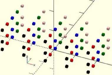
 example for() nested 3 deep

 color_vec = ["black","red","blue","green","pink","purple"];
 for (x = [-20:10:20] )
 for (y = [0:4] )color(color_vec[y])
 for (z = [0,4,10] )
     {translate([x,y*5-10,z])cube();}

 shorthand nesting for same result

 color_vec = ["black","red","blue","green","pink","purple"];
 for (x = [-20:10:20],
 y = [0:4],
 z = [0,4,10] )
     translate([x,y*5-10,z]){color(color_vec[y])cube();}
- Examples using vector of vectors
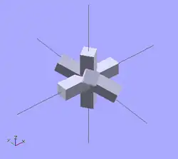
example 1 - iteration over a vector of vectors (rotation)

 for(i = [ [  0,  0,   0],
           [ 10, 20, 300],
           [200, 40,  57],
           [ 20, 88,  57] ])
{
   rotate(i)
   cube([100, 20, 20], center = true);
}
example 2 - iteration over a vector of vectors (translation)

for(i = [ [ 0,  0,  0],
          [10, 12, 10],
          [20, 24, 20],
          [30, 36, 30],
          [20, 48, 40],
          [10, 60, 50] ])
{
   translate(i)
   cube([50, 15, 10], center = true);
}
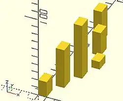
example 3 - iteration over a vector of vectors
for(i = [ [[ 0,  0,  0], 20],
          [[10, 12, 10], 50],
          [[20, 24, 20], 70],
          [[30, 36, 30], 10],
          [[20, 48, 40], 30],
          [[10, 60, 50], 40] ])
{
  translate([i[0][0], 2*i[0][1], 0])
  cube([10, 15, i[1]]);
}
Intersection For Loop
Iterate over the values in a range or vector and create the intersection of objects created by each pass.
Besides creating separate instances for each pass, the standard for() also groups all these instances creating an implicit union. intersection_for() is a work around because the implicit union prevents getting the expected results using a combination of the standard for() and intersection() statements.
intersection_for() uses the same parameters, and works the same as a For Loop, other than replacing the implicit union with an intersection.
| example 1 - loop over a range: | ||
intersection_for(n = [1 : 6])
{
    rotate([0, 0, n * 60])
    {
        translate([5,0,0])
        sphere(r=12);
    }
}
|
 |
for()_example1.jpg) |
| example 2 - rotation : | ||
 intersection_for(i = [ [  0,  0,   0],
 			[ 10, 20, 300],
 			[200, 40,  57],
 			[ 20, 88,  57] ])
{
    rotate(i)
    cube([100, 20, 20], center = true);
}
|
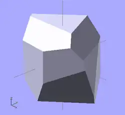 |
for()_example_2.jpg) |
If Statement
A module that evaluates an expression as a boolean value and then selects which of its children to invoke. The first child is written normally following the if() with the optional second child following the keyword "else".
if (test) doWhenTrue
if (test) doWhenTrue else doWhenFalse
As with any module, the child of an if(), or of an else, may be a block of statements in braces:
if (test) { one(); two(); x=12 }
if (test) {some=4;thing=5} else {some="a";thing="b";else="c"}
which may be empty to act as placeholders:
if (a==4) {} else echo("a is not 4");
- Parameters
- test: Usually a boolean expression, but can be any value or variable.
- See here for true or false state of values.
- See here for boolean and logical operators
- Do not confuse the assignment operator '=' with the equal operator '=='
- doWhenTrue: expression to perform when true.
- doWhenFalse: expression to perform when false.
- test: Usually a boolean expression, but can be any value or variable.
| expression | Description |
|---|---|
| b==a | true when values match |
| a<b | true when a is less than b |
| a&&b | true when both a and b are true |
| (a>=5)&&(a<=8) | a is within the range 5-8 |
Functional Examples
if( true )
    cube(4);

if( false)
    sphere(5);
else
    cube(5);
The code generated is shown by doing Design > Display CSG Tree...
group() {
    cube(size = [4, 4, 4], center = false);
}
group() {
  cube(size = [5, 5, 5], center = false);
}
Note that code is only generated for the parts of an if() for which the test is true.
If the true value in the first if() was changed to false there would be nothing in the model's tree from that statement.
If Else as Switch
Other languages may have a way to select between a number of actions based on a selector variable:
      if(test=="a") {scope1}
 else if(test=="b") {scope2}
 else if(test=="c") {scope3}
 else if(test=="d") {scope4}
 else               {scope5} // default action when test is out of range "a":"d"
Code will be generated only for the statements in the selected scope. Of course, the conditional test may be any expression:
if( (k>8)&&(k<100) ) cube(10);
else if(y==6)       {sphere(6);cube(10);}
else                 echo("any other condition");
Conditional ?: Operator
A ternary function that uses a test to determine which of 2 expressions to do.
 a =   test ? doWhenTrue : doWhenFalse;
 echo( test ? doWhenTrue : doWhenFalse);
It works like the ?: operator in other languages like 'C' or Java.
- Parameters
- test: Usually a boolean expression, but can be any value or variable.
- See here for true or false state of values.
- See here for boolean and logical operators
 Tip: Do not confuse assignment '=' with equal '=='
- doWhenTrue: the expression to do when test evaluates to true.
- doWhenFalse: the expression to do when test evaluates to false
- test: Usually a boolean expression, but can be any value or variable.
Note: The true and false expressions may not define variables using assignment, '='. A syntax error will be emitted.
- Examples
 a=1; b=2; c= a==b ? 4 : 5 ;            //  returns the number '5'
 a=1; b=2; c= a==b ? "a==b" : "a!=b" ;  //  returns the string "a!=b"

 a=5; test = a==1;           // save boolean result
 echo( test ? true: false ); // false

 L = 75; R = 2; test = (L/R)>25;
 TrueVector  = [test,L,R,L/R,cos(30)];   // define the true vector
 FalseVector = [test,L,R,sin(15)];       // define the false vector
 a1 = test ? TrueVector: FalseVector;    // [true, 75, 2, 37.5, 0.866025]
Recursive function calls
The Conditional "?:" operator is of particular use in terminating a recursion.
Note: There is a limit for recursion to prevent an application crash. When a function or module calls itself enough times the function returns undef.
Some forms of tail-recursion elimination are supported.
- Example
A function to sum the values in a vector from the Start index to the End index. When the 's' is not given it will default to zero, the first element of the vector, and the 'e' argument must be given by name. When the end index, 'e', is not given the let sets the local index, 'i', to the last index of the vector.
v = [10,20,30,40];
function sumv(v, s=0, e=undef) =
    let( i = is_undef( e ) ? len(v)-1 : e )
    i == s ?
        v[i]
    : v[i] + sumv(v, s, i-1 )
    ;

echo( sumv( v, 0, len(v)-1) );   // 100
echo( sumv( v ) );               // 100
echo( sumv( v, 1, 2 ) );         //  50
Formatting complex usage
Multiple nested conditionals can become difficult to understand. Formatting them like multi-line indented "if/else" statements is clearer.
// find the maximum value in a vector
function maxv(v, m=-999999999999, i=0) =
    (i == len(v) )
    ?     m
    :     (m > v[i])
          ?    maxv(v, m, i+1)
          :    maxv(v, v[i], i+1);

v=[7,3,9,3,5,6];
echo("max",maxv(v));   // ECHO: "max", 9
Assign Statement
[Deprecated: assign() will be removed in a future release. Use Let() instead]
Set variables to a new value for a sub-tree.
- Parameters
- The variables that should be (re-)assigned
- example:
for (i = [10:50])
{
    assign (angle = i*360/20, distance = i*10, r = i*2)
    {
        rotate(angle, [1, 0, 0])
        translate([0, distance, 0])
        sphere(r = r);
    }
}
for (i = [10:50])
{
    angle = i*360/20;
    distance = i*10;
    r = i*2;
    rotate(angle, [1, 0, 0])
    translate([0, distance, 0])
    sphere(r = r);
}
Let Statement
[Note: Requires version 2019.05]
Set variables to a new value for a sub-tree. The parameters are evaluated sequentially and may depend on each other (as opposed to the deprecated assign() statement).
- Parameters
- The variables that should be set
- example:
for (i = [10:50])
{
    let (angle = i*360/20, r= i*2, distance = r*5)
    {
        rotate(angle, [1, 0, 0])
        translate([0, distance, 0])
        sphere(r = r);
    }
}
Mathematical Operators
Scalar Arithmetic Operators
The scalar arithmetic operators take numbers as operands and produce a new number.
| + | add |
| - | subtract |
| * | multiply |
| / | divide |
| % | modulo |
| ^ | exponent [Note: Requires version 2021.01] |
The - can also be used as prefix operator to negate a number.
Prior to version 2021.01, the builtin mathematical function pow() is used instead of the ^ exponent operator.
- Example:
a=[ for(i=[0:10]) i%2 ];
echo(a);//ECHO: [0, 1, 0, 1, 0, 1, 0, 1, 0, 1, 0]
A number modulo 2 is zero if even and one if odd.
Binary arithmetic
[Note: Requires version Development snapshot]
| | | OR |
| & | AND |
| << | Left shift |
| >> | Right shift (sign preserving) |
| ~ | Unary NOT |
Numbers are converted to 64-bit signed integers for binary arithmetic, and then converted back. Note that OpenSCAD numbers have 53 bits of precision; binary arithmetic exceeding 2^53 will be imprecise.
Relational Operators
Relational operators produce a boolean result from two operands.
| < | less than |
| <= | less or equal |
| == | equal |
| != | not equal |
| >= | greater or equal |
| > | greater than |
If both operands are simple numbers, the meaning is self-evident.
If both operands are strings, alphabetical sorting determines equality and order. E.g., "ab" > "aa" > "a".
If both operands are Booleans, true > false. In an inequality comparison between a Boolean and a number true is treated as 1 and false is treated as 0. Other inequality tests involving Booleans return false.
If both operands are vectors, an equality test returns true when the vectors are identical and false otherwise. Inequality tests involving one or two vectors always return false, so for example [1] < [2] is false.
Dissimilar types always test as unequal with '==' and '!='. Inequality comparisons between dissimilar types, except for Boolean and numbers as noted above, always result in false. Note that [1] and 1 are different types so [1] == 1 is false.
undef doesn't equal anything but undef. Inequality comparisons involving undef result in false.
nan doesn't equal anything (not even itself) and inequality tests all produce false. See Numbers.
Logical Operators
All logical operators take Booleans as operands and produce a Boolean. Non-Boolean quantities are converted to Booleans before the operator is evaluated.
| && | logical AND |
| || | logical OR |
| ! | logical unary NOT |
Since [false] is true, false || [false] is also true.
Logical operators deal with vectors differently than relational operators:
[1, 1] > [0, 2] is false, but
[false, false] && [false, false] is true.
Conditional Operator
The ?: operator can be used to conditionally evaluate one or another expression. It works like the ?: operator from the family of C-like programming languages.
| ? : | Conditional operator |
| Usage Example: |
a=1;
b=2;
c= a==b ? 4 : 5;
If a equals b, then c is set to 4, else c is set to 5.
|
Vector-number operators
The vector-number operators take a vector and a number as operands and produce a new vector.
| * | multiply all vector elements by number |
| / | divide all vector elements by number |
- Example
L = [1, [2, [3, "a"] ] ];
echo(5*L);
// ECHO: [5, [10, [15, undef]]]
Vector Operators
The vector operators take vectors as operands and produce a new vector.
| + | add element-wise |
| - | subtract element-wise |
The - can also be used as prefix operator to element-wise negate a vector.
- Example
L1 = [1, [2, [3, "a"] ] ];
L2 = [1, [2, 3] ];
echo(L1+L1); // ECHO: [2, [4, [6, undef]]]
echo(L1+L2); // ECHO: [2, [4, undef]]
Using + or - with vector operands of different sizes produce a result vector that is the size of the smaller vector.
Vector Dot-Product Operator
If both operands of multiplication are simple vectors, the result is a number according to the linear algebra rule for dot product.
c = u*v; results in . If the operands' sizes don't match, the result is undef.

Matrix Multiplication
If one or both operands of multiplication are matrices, the result is a simple vector or matrix according to the linear algebra rules for matrix product. In the following, A, B, C... are matrices, u, v, w... are vectors. Subscripts i, j denote element indices.
For A a matrix of size n × m and
B a matrix of size m × p, their product
C = A*B; is a matrix of size n × p with elements
.

C = B*A; results in undef unless n = p.
For A a matrix of size n × m and
v a vector of size m, their product
u = A*v; is a vector of size n with elements
.

In linear algebra, this is the product of a matrix and a column vector.
For v a vector of size n and
A a matrix of size n × m, their product
u = v*A; is a vector of size m with elements
.

In linear algebra, this is the product of a row vector and a matrix.
Matrix multiplication is not commutative: , .


Mathematical Functions
Miscellaneous Functions
concat
[Note: Requires version 2015.03]
Concatenation function. Combine the given arguments, in the order given, to make a vector.
Input vectors are reduced to their elements in the new vector so if a given vector should be retained in the result it needs to be wrapped in square brackets ("[]").
Usage examples:
concat( 1, "string", [ 1,2], ["abc","def"])
// ECHO: [1, "string", 1, 2, "abc", "def"], ["xxx", "yyy"]
concat( [["xxx", "yyy"]], [[1,2,3]] )
// ECHO: [["xxx", "yyy"], [1, 2, 3]]
len
Length function.
Returns the length of a given vector or string.
Returns undef given any other type of input, and emits a warning.
Usage examples:
str1="abcdef"; len_str1=len(str1);
echo(str1,len_str1);

array1=[1,2,3,4,5,6,7,8]; len_array1=len(array1);
echo(array1,len_array1);

array2=[[0,0],[0,1],[1,0],[1,1]]; len_array2=len(array2);
echo(array2,len_array2);

len_array2_2=len(array2[2]);
echo(array2[2],len_array2_2);
Results:
ECHO: "abcdef", 6
ECHO: [1, 2, 3, 4, 5, 6, 7, 8], 8
ECHO: [[0, 0], [0, 1], [1, 0], [1, 1]], 4
ECHO: [1, 0], 2
Only data structures have a length:
echo( len(6) );
// WARNING: len() parameter could not be converted ...
ECHO: undef
let Module
[Note: Requires version 2015.03]
Sequential definition of temporary variables that will be local in the scope of an expression following the let().
Module Form
let( var1 = <expression>, var2 = f(<args>)) x = var1 * var2;
Usage example:
x = let(var1=23,var2=45) var1 * var2;
echo( var1, var2, x );
//WARNING: Ignoring unknown variable "var1" in file ., line 2
//WARNING: Ignoring unknown variable "var2" in file ., line 2
//ECHO: undef, undef, 1035
Let can also be used to create local variables in a Function, or in the body of a for statement.
lookup
Look up value in table, and linearly interpolate if there's no exact match. The first argument is the value to look up. The second is the lookup table -- a vector of key-value pairs.
Parameters
- key
- A lookup key
- <key,value> array
- keys and values
There is a bug in which out-of-range keys return the first value in the list. Newer versions of Openscad should use the top or bottom end of the table as appropriate instead.
Usage example: Create a 3D chart made from cylinders of different heights.
 function get_cylinder_h(p) = lookup(p, [
 		[ -200, 5 ],
 		[ -50, 20 ],
 		[ -20, 18 ],
 		[ +80, 25 ],
 		[ +150, 2 ]
 	]);

 for (i = [-100:5:+100]) {
 	// echo(i, get_cylinder_h(i));
 	translate([ i, 0, -30 ]) cylinder(r1 = 6, r2 = 2, h = get_cylinder_h(i)*3);
 }
|
 |
Generator Functions
rands
Generates a vector of pseudo random numbers greater than, or equal to, the given minimum and less than the maximum floating point values. The values in the vector will have a fractional component.
Parameters
- 1) min_value
- Required float. Minimum value of random number range
- 2) max_value
- Required float. Maximum value of random number range
- 3) value_count
- Required integer. Quantity of numbers to generate. Value taken as floor( value_count ) to remove fraction.
- seed_value
- Optional float. Seed value for random number generator for repeatable results. On versions before late 2015, seed_value gets rounded to the nearest integer.
Usage examples
// a single random number
single_rand = rands(0,10,1)[0];
echo(single_rand);
// a vector of 4 numbers between 5 and 15
seed=42;
random_vect=rands(5,15,4,seed);
echo( "Vector: ",random_vect);
sphere(r=5);
for(i=[0:3]) {
 rotate(360*i/4) {
   translate([10+random_vect[i],0,0])
     sphere(r=random_vect[i]/2);
 }
}
// ECHO: "Vector: ", [8.7454, 12.9654, 14.5071, 6.83435]
To obtain random integers between 1 and 10 inclusive we note that rands(1,10,...) only spans 9 values so the results will be mostly fractional.
To properly generate integer values in the desired range the parameters should be set to generate right number of intervals.
function irands(minimum, maximum, n) =
    let(floats = rands(minimum, maximum+1, n))
    [ for (f = floats) floor(f) ];
echo(irands(1, 10, 5));
// ECHO: [9, 6, 2, 4, 1]
Mathematical Functions
abs
Mathematical absolute value function. Returns the positive value of the given number.
Usage examples:
abs(-5.0);  returns 5.0
abs(0);     returns 0.0
abs(8.0);   returns 8.0
ceil
Mathematical ceiling function. Returns the next largest integer value as described elsewhere.
Usage examples:
echo(ceil(4.4),ceil(-4.4)); // produces ECHO: 5, -4
cross
Calculates the cross product of two vectors.
Both vectors must be the same length, with either three or two values, or the function returns undef.
The cross product of 3D vectors is a vector that is perpendicular to its inputs.
With 2D vectors the cross product can only have a value in the third position of the vector, [0,0,z] which is its determinant.
In this case the cross() function returns just the determinant value, the z value of the vector:
cross([x,y,z], [u,v,w]) --> [ x*v, y*u, z*w ]
cross([x,y], [u,v]) --> x*v - y*u --> d
For any two vectors, 2D or 3D, the following holds for vectors a and b:
cross(a,b) == -cross(b,a)
Usage examples:
echo(cross([2, 3, 4], [5, 6, 7]));     // produces ECHO: [-3, 6, -3]
echo(cross([2, 1, -3], [0, 4, 5]));    // produces ECHO: [17, -10, 8]
echo(cross([2, 1], [0, 4]));           // produces ECHO: 8
echo(cross([1, -3], [4, 5]));          // produces ECHO: 17
echo(cross([2, 1, -3], [4, 5]));       // produces ECHO: undef
exp
Mathematical exponent function using base e.
Returns ex, the exponential function of x,
echo(exp(1),exp(ln(3)*4)); // produces ECHO: 2.71828, 81
floor
Mathematical floor function. Returns the integer equal to, or smaller than the given value, as described elsewhere
echo(floor(4.4),floor(-4.4)); // produces ECHO: 4, -5
ln
The mathematical natural logarithm of x is the power to which e would have to be raised to equal x. Normally written as ln x or, to make the base e explicit, loge x as explained in Natural logarithm
log
Base-10 logarithm of a number. The mathematical logarithm of a number is the exponent by which another fixed value, the base, must be raised to produce that number; see w:Logarithm.
y = log(1000); // returns 3, because 103 = 1000
max
Returns the maximum of the parameters.
Given a single vector the function returns the element with the maximum value.
Any other data type emits a warning and returns undef.
Function's Forms
- max(n{,n}*)
- one or more floating values
- max( [n{,n}*] )
- a single vector of one or more floating values
Usage example:
max(3.0,5.0);   // 5.0
max(-11,-22);   // -11
max([8,3,4,5]); // 8
min
Returns the minimum of the parameters. Given a single vector the function returns the element with the minimum value.
Function's Forms
- min(n{,n}*)
- one or more floating values
- min( [n{,n}*] )
- a single vector of one or more floating values
Usage example:
min(3.0,5.0);   // 3.0
min(-11,-22);   // -22
min([8,3,4,5]); // 3
mod
The modulo operation is implemented as an operator that takes two arguments, as described in the section on the modulo operator (%).
It is mentioned here to make clear that OpenSCAD does not provide a mod() function,
norm
Returns the Euclidean norm of a vector:

This returns the actual numeric length while len() returns the number of elements in the vector or array.
Usage examples:
a=[1,2,3,4,5,6];
b="abcd";
c=[];
d="";
e=[[1,2,3,4],[1,2,3],[1,2],[1]];
echo(norm(a)); //9.53939
echo(norm(b)); //undef
echo(norm(c)); //0
echo(norm(d)); //undef
echo(norm(e[0])); //5.47723
echo(norm(e[1])); //3.74166
echo(norm(e[2])); //2.23607
echo(norm(e[3])); //1
Results:
ECHO: 9.53939
ECHO: undef
ECHO: 0
ECHO: undef
ECHO: 5.47723
ECHO: 3.74166
ECHO: 2.23607
ECHO: 1
pow
Mathematical power function that raises the base to the power of the exponent.
As of version 2021.01 you can use the exponentiation operator ^ instead.
Parameters
- <base>
- Decimal. Base.
- <exponent>
- Decimal. Exponent.
Usage examples:
for (i = [0:5]) {
 translate([i*25,0,0]) {
   cylinder(h = pow(2,i)*5, r=10);
   echo (i, pow(2,i));
 }
}
echo(pow(10,2)); // 10^2 or 10*10
// result: ECHO: 100

echo(pow(10,3)); // 10^3 or 10*10*10
// result: ECHO: 1000
echo(pow(125,1/3)); // means 125^(0.333...), the cube root of 125
// result: ECHO: 5
round
The round function returns the integer value of given .
Usage examples:
round(5.4);  //  5
round(5.5);  //  5
round(5.6);  //  6
round(-5.4); // -5
round(-5.5); // -6
round(-5.6); // -6
Rounding to the nearest value v involves multiplying the argument of round() by 1/v and dividing the result of round() by 1/v. For example, round(x/6)*6 rounds the value x to the nearest multiple of 6, round(x*10)/10 rounds the value x to the nearest multiple of 0.1.
sign
Mathematical sign function. Returns a signed unit value, thus one (1), with the same sign as the given value, or zero (0) when the input is zero, as explained elsewhere
Parameters
- <x>
- Decimal. Value to find the sign of.
Usage examples:
sign(-5.0);   // -1
sign(0);      //  0
sign(8.0);    //  1
sqrt
Mathematical square root function.
- Usage example
translate([sqrt(100),0,0])sphere(100);
String Functions
str
Convert all arguments to strings and concatenate.
Usage examples:
number=2;
echo ("This is ",number,3," and that's it.");
echo (str("This is ",number,3," and that's it."));
Results:
ECHO: "This is ", 2, 3, " and that's it."
ECHO: "This is 23 and that's it."
This can be used for simple conversion of numbers to strings
s = str(n);
chr
[Note: Requires version 2015.03]
Convert numbers to a string containing character with the corresponding code. OpenSCAD uses Unicode, so the number is interpreted as Unicode code point. Numbers outside the valid code point range produce an empty string.
Parameters
- chr(Number)
- Convert one code point to a string of length 1 (number of bytes depending on UTF-8 encoding) if the code point is valid.
- chr(Vector)
- Convert all code points given in the argument vector to a string.
- chr(Range)
- Convert all code points produced by the range argument to a string.
Examples
echo(chr(65), chr(97));      // ECHO: "A", "a"
echo(chr(65, 97));           // ECHO: "Aa"
echo(chr([66, 98]));         // ECHO: "Bb"
echo(chr([97 : 2 : 102]));   // ECHO: "ace"
echo(chr(-3));               // ECHO: ""
echo(chr(9786), chr(9788));  // ECHO: "☺", "☼"
echo(len(chr(9788)));        // ECHO: 1
Note: When used with echo() the output to the console for character codes greater than 127 is platform dependent.
ord
[Note: Requires version 2019.05]
Convert a character to a number representing the Unicode code point. If the parameter is not a string, the ord() returns undef.
Parameters
- ord(String)
- Convert the first character of the given string to a Unicode code point.
Examples
echo(ord("a"));
// ECHO: 97

echo(ord("BCD"));
// ECHO: 66

echo([for (c = "Hello! 🙂") ord(c)]);
// ECHO: [72, 101, 108, 108, 111, 33, 32, 128578]

txt="1";
echo(ord(txt)-48,txt);
// ECHO: 1,"1" // only converts 1 character
len
returns the number of characters in a text.
echo(len("Hello world")); // 11
See Also search()
search() for text searching.
is_string( <variable> )
The function is_string(value) return true if the value is a string, false else
echo(is_string("alpha")); //true
echo(is_string(22)); //false
Trigonometric functions
The trig functions use the C Language mathematics functions, which are based in turn on Binary Floating Point mathematics, which use approximations of Real Numbers during calculation. OpenSCAD's math functions use the C++ 'double' type, inside Value.h/Value.cc,
A good resource for the specifics of the C library math functions, such as valid inputs/output ranges, can be found at the Open Group website math.h & acos
cos
Mathematical cosine function of degrees. See Cosine
Parameters
- <degrees>
- Decimal. Angle in degrees.
| Usage example: | |
 for(i=[0:36])
    translate([i*10,0,0])
       cylinder(r=5,h=cos(i*10)*50+60);
|
 |
sin
Mathematical sine function. See Sine
Parameters
- <degrees>
- Decimal. Angle in degrees.
| Usage example 1: | |
 for (i = [0:5]) {
  echo(360*i/6, sin(360*i/6)*80, cos(360*i/6)*80);
   translate([sin(360*i/6)*80, cos(360*i/6)*80, 0 ])
    cylinder(h = 200, r=10);
 }
|
| Usage example 2: | |
 for(i=[0:36])
    translate([i*10,0,0])
       cylinder(r=5,h=sin(i*10)*50+60);
|
 |
tan
Mathematical tangent function. See Tangent
Parameters
- <degrees>
- Decimal. Angle in degrees.
| Usage example: | |
 for (i = [0:5]) {
  echo(360*i/6, tan(360*i/6)*80);
   translate([tan(360*i/6)*80, 0, 0 ])
    cylinder(h = 200, r=10);
 }
|
acos
Mathematical arccosine, or inverse cosine, expressed in degrees. See: Inverse trigonometric functions
asin
Mathematical arcsine, or inverse sine, expressed in degrees. See: Inverse trigonometric functions
atan
Mathematical arctangent, or inverse tangent, function. Returns the principal value of the arc tangent of x, expressed in degrees. atan cannot distinguish between y/x and -y/-x and returns angles from -90 to +90. See: atan2 and also Inverse trigonometric functions
atan2
Mathematical two-argument atan function atan2(y,x) that spans the full 360 degrees. This function returns the full angle between the x axis and the vector(x,y) expressed in degrees, in the range .

Usage examples:
atan2(5.0,-5.0);     //result: 135 degrees. atan() would give -45
atan2(y,x);          //angle between (1,0) and (x,y) = angle around z-axis
String Functions
String Functions
str
Convert all arguments to strings and concatenate.
Usage examples:
number=2;
echo ("This is ",number,3," and that's it.");
echo (str("This is ",number,3," and that's it."));
Results:
ECHO: "This is ", 2, 3, " and that's it."
ECHO: "This is 23 and that's it."
This can be used for simple conversion of numbers to strings
s = str(n);
chr
[Note: Requires version 2015.03]
Convert numbers to a string containing character with the corresponding code. OpenSCAD uses Unicode, so the number is interpreted as Unicode code point. Numbers outside the valid code point range produce an empty string.
Parameters
- chr(Number)
- Convert one code point to a string of length 1 (number of bytes depending on UTF-8 encoding) if the code point is valid.
- chr(Vector)
- Convert all code points given in the argument vector to a string.
- chr(Range)
- Convert all code points produced by the range argument to a string.
Examples
echo(chr(65), chr(97));      // ECHO: "A", "a"
echo(chr(65, 97));           // ECHO: "Aa"
echo(chr([66, 98]));         // ECHO: "Bb"
echo(chr([97 : 2 : 102]));   // ECHO: "ace"
echo(chr(-3));               // ECHO: ""
echo(chr(9786), chr(9788));  // ECHO: "☺", "☼"
echo(len(chr(9788)));        // ECHO: 1
Note: When used with echo() the output to the console for character codes greater than 127 is platform dependent.
ord
[Note: Requires version 2019.05]
Convert a character to a number representing the Unicode code point. If the parameter is not a string, the ord() returns undef.
Parameters
- ord(String)
- Convert the first character of the given string to a Unicode code point.
Examples
echo(ord("a"));
// ECHO: 97

echo(ord("BCD"));
// ECHO: 66

echo([for (c = "Hello! 🙂") ord(c)]);
// ECHO: [72, 101, 108, 108, 111, 33, 32, 128578]

txt="1";
echo(ord(txt)-48,txt);
// ECHO: 1,"1" // only converts 1 character
len
returns the number of characters in a text.
echo(len("Hello world")); // 11
See Also search()
search() for text searching.
is_string( <variable> )
The function is_string(value) return true if the value is a string, false else
echo(is_string("alpha")); //true
echo(is_string(22)); //false
List Comprehensions
[Note: Requires version 2015.03]
Syntax of List comprehensions
List comprehensions are a powerful tool for generating lists using the syntax:
[ list-definition-element* ]
meaning that there may be one or more comma separated elements inside the square brackets each of which may be one of these generators:
- <literal>
- any literal number, string, vector
- <expression>
- any normal arithmetic, logical, expression or function call
- for( i = [start:incr:end] )
- Iteration over a range, same as
for loop - for( i = vector )
- over an existing list, same as
for loop - for( i = "string")
- over an existing string, same as
for loop - for( init;condition;next )
- C-style
forloop, each section minimum one expression.[Note: Requires version 2019.05] Note: not available as a statement , see below. - each
- unpacks following vectors, or ranges, and adds each element to the list being constructed
- if( <condition> ) <expression>
- when condition is false, nothing is added to the list, otherwise the <expression> is evaluated and its result becomes a list element
- if( <condition> ) <expression> else <expression>
- when <condition> is true, the first expression is evaluated and its result becomes a list element, otherwise the second expression is used.
The let( localvar = <expression> ) statement deserves special mention for its role allowing calculations to be done in the scope of the for loop's body.
But it is not properly a generator.
Note: in OpenSCAD vector and list are synonyms for the data structure delimited by square brackets "[]". The term "array" is also synonymous, but is used more in other languages than this one.
Multiple Generator Expressions
[Note: Requires version 2019.05]
There is no restriction on the expressions used to build a list.
Specifically, for loop generators are effectively expressions that return a number of list elements and more than one may be used so long as they are separated from one another by a comma ",".
steps = 50;
points = [
	// generating points in +Y
	for (a = [0 : steps]) [ a, 10 * sin(a * 360 / steps) + 10 ],
	// generating in -Y
	for (a = [steps : -1 : 0]) [ a, 10 * cos(a * 360 / steps) - 20 ],
	// also add three more points
	[ 10, -3 ],
    func_returning_list(a,b,true),
    x+2*y
    ];
polygon(points);
For Element
The for element uses the same syntax the for loop statement.
At least one loop index variable must be named and they operate as local variables in the body the for loop.
The for loop may be nested in two ways, by setting more than one index, or by nesting them:
x = [ for( i=[1,2,3], j="acb") each [i,j] ];
y = [ for( i=[1,2,3] ) for( j=i ) each [i,j] ];
A range may be used to generate a sequential list:
list1 = [ for (i = [0 : 2 : 10]) i ];
echo(list1); // ECHO: [0, 2, 4, 6, 8, 10]
A range may be used to selectively extract items from string or vector:
str = "I1n2t3e4r5e6s7t8i9n0g";
list = [ for (i = [0 : 2 : len(str) - 1]) str[i] ];
echo( list );
// ECHO:  ["I", "n", "t", "e", "r", "e", "s", "t", "i", "n", "g"]
To generate an irregular sequence of list values a commonly used tactic is to put the irregular items into a list that is then used to calculate the needed values:
function func(x) = x < 1 ? 0 : x + func(x - 1);
inputs= [1, 3, 5, 8];
output = [for(a = inputs) func(a) ];
echo(output); // ECHO: [1, 6, 15, 36]
Iterate over an existing list to output lengths of string elements:
friends = ["John", "Mary", "Alice", "Bob"];
list = [ for (i = friends) len(i)];
echo(list); // ECHO: [4, 4, 5, 3]
Generate a list by looping over the characters of a string. [Note: Requires version 2019.05]
echo([ for (c = "String") c ]);
// ECHO: ["S", "t", "r", "i", "n", "g"]
Multi-section For Loop
[Note: Requires version 2019.05]
This list generator expression follows the syntax of the C Language for loop in that it has three sections in is control structure:
- initialization
- comma separated list of assignment expressions, as
a=<expr> - ending condition expression
- a single expression resulting in a boolean. When the expression evaluates to
falsethe loop terminates. - increment section
- comma separated list of assignment expressions, as
a=<expr>where each variable in the initialization list is modified to the value wanted in the next iteration. A simple form of update is :a=a+1but any expression or function call may be used.
[for(a=0,i=12,exit=false ; a<10 || exit ; a=a+1, i=newIndex(i) )
  exit = calc_an_element( a, i )
  ]
There are some issues of scope to pay attention to:
x = [for(a=0,i=12,exit=false; a<10 && !exit ; a=a+1, i=+12, exit = a==5 )
 a*i
 ];
echo(x);
returns x as this vector [0, 12, 24, 36, 48] as "exit" is made false at a==5.
But in this:
x = [for(a=0,i=12,exit=false; a<10 && !exit ; a=a+1, i=+12/*no exit*/ )
 let(exit = a==5)
 a*i
 ];
echo(x);
the local variable, "exit" inside for(-*-) is not visible in the body of the loop, so the let statement is creating a completely new local called "exit".
The vector x is now ECHO: [0, 12, 24, 36, 48, 60, 72, 84, 96, 108]
Note: This form of the for loop is only for list initialization. It not be used in a for loop statement
Generate a vector of [X,Y] position vectors:
echo( [for (a = 0, b = 1;a < 5;a = a + 1, b = b + 2) [ a, b * b ] ] );
// ECHO: [[0, 1], [1, 9], [2, 25], [3, 49], [4, 81]]
Generate Fibonacci sequence
echo([for (a = 0, b = 1;a < 1000;x = a + b, a = b, b = x) a]);
// ECHO: [0, 1, 1, 2, 3, 5, 8, 13, 21, 34, 55, 89, 144, 233, 377, 610, 987]
A useful tactic is to use the versatility of the multi-section for initializer to generate a vector of which only the last value is wanted. For instance, a loop can keep a rolling sum as it goes, resulting in a vector of sums. To obtain the cumulative sum of all the values:
function cumsum(v) = [for (a = v[0]-v[0], i = 0; i < len(v); a = a+v[i], i = i+1) a+v[i]]; echo(cumsum([1, 2, 3, 4])); //ECHO: [1, 3, 6, 10]
Changing this slightly:
function cumsum(v) =
let( sum=[for (a = v[0]-v[0], i = 0; i < len(v); a = a+v[i], i = i+1)
a+v[i]] )
sum[len(sum)-1]
;
echo( cumsum([10,20,30]) ); //ECHO: 60
the accumulated value we want is in the last element of the vector so we return that and discard the temporary vector.
A recursive function may be written to process a vector in the same way:
function f(a, b, ...) =
condition ?
concat([expr], f(nexta, nextb, ...))
: [];
f(inita, initb, ...)
The concat() function is needed to join the element [expr] with the rest of the vector that will be returned from the function f.
Each Element
[Note: Requires version 2019.05]
The each element acts to "flatten" the generator that follows it to simplify the resulting vector.
Generate a nested list of vectors:
echo( [ for (a = [1 : 4]) [a, a*a] ] ); // ECHO: [[1, 1], [2, 4], [3, 9], [4, 16]]
Using "each" produces a flat list by extracting the values of the inner vector and adding them to the resulting vector directly:
echo([ for (a = [1 : 4]) each [a, a*a] ]); // ECHO: [1, 1, 2, 4, 3, 9, 4, 16]
Each just needs to be in front of the vectors to be simplified:
echo([ each for (a = [1 : 4]) [a, a*a] ]); // ECHO: [1, 1, 2, 4, 3, 9, 4, 16]
Remembering that each is a generator just like the for loop variants:
echo( [each [1,2,3,4], [1,2,3,4] ] ); // ECHO: [1, 2, 3, 4, [1, 2, 3, 4]]
echo( [each [1,2,3,4], each[1,2,3,4] ] ); // ECHO: [1, 2, 3, 4, 1, 2, 3, 4]
echo( [each [ [1,2,3,4], [1,2,3,4] ] ] ); // ECHO: [[1, 2, 3, 4], [1, 2, 3, 4]]
each can also be applied to a range to expand the sequence and insert its values as list element:
echo( [each [1:2:5]] ); //ECHO: [1,3,5]
or
echo( [each [6:-2:0]] ); //ECHO: [6, 4, 2, 0]
if Element
The if element may be used to check if a calculated result should be added to the list or not. In obvious use case is filtering unwanted items from a list.
[ for() if (condition()) i ] : When the condition is true, the i is added to the list.
list = [ for (a = [ 1 : 8 ]) if (a % 2 == 0) a ];
echo(list); // ECHO: [2, 4, 6, 8]
The if element must follow the closing parenthesis of for(), with the exception that a let() statement may be inserted to define some locals.
list = [-10:5]; x=[for(n=list) let(y=2) if(n%2==0 || n>=0) n%2==0 ? n/2 : n*y ]; echo(x);
Giving
ECHO: [-5, -4, -3, -2, -1, 0, 2, 1, 6, 2, 10]
if-else Element
[Note: Requires version 2019.05] This element adds the possibility for different expressions on each side of a decision.
[ for (i = list) if (condition(i)) x else y ]
When the condition is true, x is added else y is.
A more complex example will make a list where even numbers are halved, positive odd numbers are preserved, negative odd numbers are eliminated:
echo([for (a = [-3:5])
if (a % 2 == 0)
[a, a/2]
else if (a > 0)
[a, a]
]);
// ECHO: [[-2, -1], [0, 0], [1, 1], [2, 1], [3, 3], [4, 2], [5, 5]];
Note that if-else may not be nested using braces but if we note that parentheses may be used to control order of evaluation. In this example even numbers are dropped, and multiples of 4 are substituted by -1
echo([for(i=[0:10]) if(i%2==0) (if(i%4==0) -1 ) else i]);
// ECHO: [-1, 1, 3, -1, 5, 7, -1, 9]
Alternatively; in this one odd numbers are dropped, multiples of 4 are substituted by -1
echo([for(i=[0:10]) if(i%2==0) if(i%4==0) -1 else i]);
// ECHO: [-1, 2, -1, 6, -1, 10]
let Statement
The elements in a let statement is a comma separated list of assignment expressions that define local variables that will only be visible in the body of the for loop.
[ for (i = list) let( <assignment>*, ) i ]
list = [ for (a = [ 1 : 4 ]) let (b = a*a, c = 2 * b) [ a, b, c ] ];
echo(list); // ECHO: [[1, 1, 2], [2, 4, 8], [3, 9, 18], [4, 16, 32]]
Nested loops
The flexibility of the looping generators allow for a variety of methods for generating vectors.
Using multiple loop variables:
flat_result1 = [ for (a = [ 0 : 2 ], b = [ 0 : 2 ])
a == b ? 1 : 0
];
echo(flat_result1); // ECHO: [1, 0, 0, 0, 1, 0, 0, 0, 1]
Nesting for loop elements:
flat_result2 = [ for (a = [ 0 : 2 ])
for (b = [0 : 2]) a == b ? 1 : 0
];
echo(flat_result2); // ECHO: [1, 0, 0, 0, 1, 0, 0, 0, 1]
Nested loops can generate matricies:
identity_matrix = [ for (a = [ 0 : 2 ])
[ for (b = [ 0 : 2 ]) a == b ? 1 : 0 ]
];
echo(identity_matrix); // ECHO: [[1, 0, 0], [0, 1, 0], [0, 0, 1]]
Advanced Examples
This chapter lists some advanced examples, useful idioms and use-cases for the list comprehension syntax.
Generating vertices for a polygon
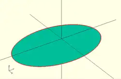
Using list comprehension, a parametric equation can be calculated at a number of points to approximate many curves, such as the following example for an ellipse (using polygon()):
sma = 20; // semi-minor axis
smb = 30; // semi-major axis
polygon(
[ for (a = [0 : 5 : 355])
[ sma * sin(a), smb * cos(a) ]
]
);
Flattening a nested vector
Defining a function to perform a task on a vector is a good way to document the calculation being performed. It is also then possible to use it to define more complex procedures with a reduced risk of introducing errors as complexity increases.
Here we take two lists and join them together:
function flatten(l) = [ for (a = l) for (b = a) b ] ;
nested_list = [ [ 1, 2, 3 ], [ 4, 5, 6 ] ];
echo(flatten(nested_list)); // ECHO: [1, 2, 3, 4, 5, 6]
The nested for loops unpack the two as the output list is processed.
The following example on concatenating lists shows a number of other way the same operation may be done.
Quicksort Using Vectors
The Quicksort algorithm may be implemented using for() and if() generators along let() and recursion:
Given as list of items that have a sorting order this function returns the same list sorted in ascending order:
function quicksort( list ) =
len(arr) <= 0 ? [] : // nothing to sort, return empty list
let(
pivot = arr[floor(len(arr)/2)],
lesser = [ for (y = arr) if (y < pivot) y ],
equal = [ for (y = arr) if (y == pivot) y ],
greater = [ for (y = arr) if (y > pivot) y ]
)
concat( quicksort(lesser), equal, quicksort(greater) )
;
// use seed in rands() to get reproducible results
unsorted = [for (a = rands(0, 10, 6, 3)) ceil(a)];
echo(unsorted); // ECHO: [6, 1, 8, 9, 3, 2]
echo(quicksort(unsorted)); // ECHO: [1, 2, 3, 6, 8, 9]
unsorted = "aqasdf19edkdz0adfga.";
echo(quicksort(unsorted));
// ECHO: [".", "0", "1", "9", "a", "a", "a", "a", "d", "d", "d", "d", "e", "f", "f", "g", "k", "q", "s", "z"]
The input list is broken into three parts, based on the pivot, the lesser, equal, and greater.
The if() filter leaves out the unwanted elements as each of the three are processed, and the result is assembled by concat().
The calls to the quicksort() function inside the concat() are the recursion elements.
Selecting elements of a vector
This user-defined select() function may be used on a given vector to extract items .. selectively.
function select(vector, indices) = [ for (index = indices) vector[index] ];
vector1 = [[0,0],[1,1],[2,2],[3,3],[4,4]];
selector1 = [4,0,3];
vector2 = select(vector1,selector1); // [[4, 4], [0, 0], [3, 3]]
vector3 = select(vector1,[0,2,4,4,2,0]);// [[0, 0], [2, 2], [4, 4],[4, 4], [2, 2], [0, 0]]
// a range also works as indices
vector4 = select(vector1, [4:-1:0]); // [[4, 4], [3, 3], [2, 2], [1, 1], [0, 0]]
Concatenating two vectors
Concatenating two OpenSCAD lists, [1,2,3] and [4,5]
function cat(L1, L2) = [for (i=[0:len(L1)+len(L2)-1])
i < len(L1)? L1[i] : L2[i-len(L1)]] ;
echo(cat([1,2,3],[4,5])); //ECHO: [1, 2, 3, 4, 5]
But the same results may be achieved using only concat() or each:
echo( concat( [1,2,3],[4,5]) ); // ditto echo( [each [1,2,3], each [4,5]]); // ditto
The list based forms also work. Note the use of the temporary L variable that concatenates the L1 and L2 vectors.
This only works inside the generator for() parentheses.
Also note that second local "a" is necessary to unpack the joined vectors:
function cat(L1, L2) = [for(L=[L1, L2], a=L) a];
This construction has the same effect as using each:
function cat3(L1, L2) = [for(L=[ each L1, each L2] ) L];
Other Language Features
Curve Smoothness: $fa, $fs, and $fn
These are three of the Special Variables defined as part of the language.
![]() Best Practice: Set $fs=0.5, $fa=1, $fn=0 for good smooth curves with reasonable performance and only use $fn > 0 to generate regular polygons.
Best Practice: Set $fs=0.5, $fa=1, $fn=0 for good smooth curves with reasonable performance and only use $fn > 0 to generate regular polygons.
The $fa, $fs values, OR the $fn value, are used to calculate how many facets a curved line or surface should be divided into, creating line segments or polygons respectively, to approximate a smoothed curve.
Smoothness Notes
- The terms fragment and facet are used interchangeably in this section.
- When $fn > 0, $fs and $fa are not used, and vice versa
- the number of facets is always an integer value.
Not Really About Rendering
These smoothness variables are actually involved in the generation of geometry, not rendering per se. Of course the generation of polygonal approximations of the mathematical shapes modeled by a script is pretty close to the rendering process. Just without rendering an image or exporting an STL file to be 3D printed.
Including this section in the Rendering page is a reflection of it being a source of rendering issues.
Using $fa and $fs
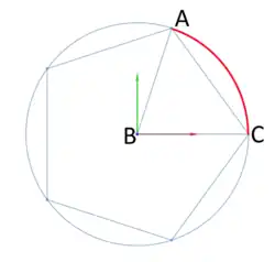
When $fa and $fs variables are being used curved objects are divided into a minimum of 5 fragments.
$fa is the minimum angle for a fragment, the angle A-B-C in the diagram, and controls the division of large circles. The minimum angle prevents a large circle being divided into microscopic facets that can't be rendered or a reproduced on a 3D printer. The default value is 12 which gives 30 fragments around a circle. The minimum value allowed is 0.01.
$fs is the minimum size of a fragment, measured in millimeters along its arc length, from A to C (in red) and controls the division of small circles. The minimum arc length prevents a circle being divided into microscopic sides, as for $fa. The default value is 2 so very small circles have a smaller number of fragments than specified using $fa. The minimum allowed value is 0.01.
The radius of curvature is factored into the fragments calculation so best practice recommendation of $fa=1 and $fs=0.5 produces smooth looking curves for a very wide range of size.
Using $fn
When greater than zero, $fn is an integer value setting the number of fragments that a curved line or surface will be divided into, to a minimum of 3. When assigned a floating point value any fractional part is truncated, thus $fn=6.89 results in 6-sided objects.
Curves will appear to be smoother as $fn is increased, but will require more memory and CPU power to render. Setting $fn >= 128 is not recommended.
![]() Best Practice: is to only use $fn to create regular polygonal shapes, leaving curve smoothness to $fa and $fs. low values for $fn may be used to create regular polygons or 3D prisms
Best Practice: is to only use $fn to create regular polygonal shapes, leaving curve smoothness to $fa and $fs. low values for $fn may be used to create regular polygons or 3D prisms
When the $fn value is divisible by 4 the polygon will be drawn on integral boundaries and be inscribed within a circle of the given diameter.
Slicing Solids
The curved 3D objects, spheres and cylinders, are divided into pie-shaped facets in the same way as circles are, and are also divided into horizontal "slices" using a similar calculation. Then, between the vertices formed by the divisions four sided polygons are drawn. The tops and bottoms are drawn as polygons with the same number of edges as there are facets.
This subdivision method is used on curved, regular shapes imported from DXF files, but is not used on 3D shapes from STL files as they are already in triangles.
Calculating Number of Fragments
This is the C code that calculates the number of fragments for a circle of radius "r":
int get_fragments_from_r(double r, double fn, double fs, double fa)
{
if (r < GRID_FINE)
return 3;
if (fn > 0.0)
return (int)(fn >= 3 ? floor(fn) : 3); // minimum 3
// which ever of $fa or $fs is used, minimum 5
return (int) ceil( fmax( fmin( 360.0 / fa, r*2*M_PI / fs), 5 ) );
}
GRID_FINE is an arbitrary constant for the smallest radius that will be accepted as an argument to the primitive generating object modules.
This is the equivalent calculation in OpenSCAD given a radius (r) for the curve:
r=10; // radius of the curve being considered
echo(
n=($fn>0?
($fn>=3? $fn : 3) :
ceil( max( min( 360/$fa, r*2*PI/$fs ), 5 ) )
),
a_based = 360/$fa,
s_based = r*2*PI/$fs
);
ECHO: n = 30, a_based = 30, s_based = 31.4159
The curvature variables may be set globally in a program:
$fs = 3.1; sphere(2);
or individually set on a primitive as a named parameter:
sphere(2, $fn = 6.4);
or modified by a scaling factor taking advantage of local scope rules:
sphere( 2, $fa = $fa*1.1 );
Viewport: $vpr, $vpt, $vpf and $vpd
These Special Variables reflect the current viewport parameters at the time of rendering.
The current viewport values may be copied onto the clipboard using the menu items Edit > Copy Viewport *.
From there it may be pasted into a script.
Changing the view interactively does not affect the special variables. During an animation they are updated for each frame.
- $vpr
- rotation vector of floats [phi-x,phi-y,phi-z] - Camera Pan, Tilt & Yaw
- $vpt
- translation vector [x,y,z] - Camera Rack, Truck & Pedestal
- $vpf
- non-negative float > 5, - Camera Zoom, set as the angle in degrees of the Field of View (FoV) [Note: Requires version 2021.01]
- $vpd
- non-negative float > 0.01, the camera distance [Note: Requires version 2015.03]
These four variables give the position and orientation of the camera, or eye point, that is used as the basis for rendering images.
Rotation Vector
The effect of rotation on the camera must always factor in the cameras base position and its distance.
With rotation set to [0,0,0] and translate=[0,0,0] the view is down the Z axis to the origin. The camera's rotation is clockwise, considered looking from the origin in the positive direction of the axis, so [0,90,0] rotates the camera "down" to the X axis, still looking at the origin.
Rotations are applied at the translated position of the camera and will appear to be reversed by the change in the viewport.
Rotating to move the view up means applying a rotation to tilt the camera down.
Likewise, to look left the camera must rotate to the right.
The effect of rotation is magnified when the Camera Distance is larger.
Translation Vector
This sets the base position of the camera in coordinate space and is not affected by rotate and zoom.
We say the base position as the camera is actually positioned the camera distance along the direction of the rotation vector from its base position.
Field of View
This is the angle, in degrees, of the viewing area of the camera. Making the FoV larger does Zoom In, and smaller values Out.
Camera Distance
A floating point value for the distance, in millimeters, from the base position to the camera, along the vector set by the rotation vector.
Example
$vpr = [0, 0, $t * 360];
causes the camera to rotate 360 degree the Z axis when animating.
Animation Using the $t Special Variable
Animation is started by selecting the Window > Animate menu item and then entering values for "FPS" and "Steps" in the Animation Panel that opens.
The "Time" field shows the current value of $t, the animation time variable, as a decimal fraction.
This variable, when active, is used in all rotate() and translate() modules, $t*360 giving complete cycles.
The value of $t will repeat from 0 through (1 - 1/Steps). It never reaches 1 because this would produce a "hitch" in the animation if using it for rotation -- two consecutive frames would be at the same angle.
There is no variable to distinguish between the cases of animation running at the first frame ($t=0) and animation not running, so make $t=0 your rest position for the model.
Render Mode: $preview
[Note: Requires version 2019.05]
This Special Variable may be interrogated to know in which rendering mode the script is being run.
When in OpenCSG preview mode (F5) $preview is true.
Doing a render (F6) it is false.
![]() Tip: $fn should not be used to globally control how curved shapes are sub-divided, $fa & $fs do a better job
Tip: $fn should not be used to globally control how curved shapes are sub-divided, $fa & $fs do a better job
The render() module operates differently from either rendering mode. The value of $preview is undetermined in this snippet:
render(){
$fn = $preview ? 12 : 72;
sphere(r = 1);
}
The tessellation result is the same regardless.
Command Line Operation
When using the command line to render $preview is only true when exporting a PNG image.
For all other forms of output ( STL, DXF, SVG, CSG, and ECHO files ) it is false.
It can be forced true using the -D command line option.
Examples
$preview can be used to model in reduced detail but have fully smoothed curved surfaces the final rendered result:
FNspecial = $preview ? 12 : 72; sphere(r = 1, $fn=FNspecial );
![]() Best Practice: The $fn argument to the module is used so that no other shapes are affected.
Best Practice: The $fn argument to the module is used so that no other shapes are affected.
Another use could be to show a complex part assembled during preview but spread out and positioned for 3D printing during rendering.
OR: When horizontal features require support in 3D printing the object may be previewed without the support structures, but rendered with them, then exported to STL for printing.
Echo
A call to echo() prints its given arguments to the compilation window (aka Console).
Any number of arguments of any type may be given, including function calls and other expressions.
Each given argument is separated by a comma and a space.
Strings are displayed in double quotes ('"'), vectors by square brackets ("[]"), and objects inside braces ("{}").
The String Function str() may be used to prepackage a number of values into a string so that values will NOT be separated by a blank. Str() also does not add quotes around strings and does not separate elements with ", ".
Numeric values are rounded off to 5 significant digits. This means that fractions smaller than 0.000001 are not displayed and that very large values are shown in scientific notation with only the first 6 digits shown.
Arguments to Echo() may be given individual labels by using the form: 'variable=variable' as will be seem in this example.
Usage examples:
my_h=50;
my_r=100;
echo("a cylinder with height : ", my_h, " and radius : ", my_r);
echo( high=my_h, rad=my_r); // will display as high=<num> rad=<num>
cylinder(h=my_h, r=my_r);
small Decimal Fractions are Rounded Off
This example shows that the fractional part of 'b' may appear to be rounded off when printed by echo(), but is still present for use in calculations and logical comparisons:
a=1.0;
b=1.000002;
echo(a); // shows as '1'
echo(b); // also shows as '1'
if(a==b){
echo ("a==b");
}else if(a>b){
echo ("a>b");
}else if(a<b){
echo ("a<b"); // will be the result
}else{
echo ("???");
}
Shows in the Console as
ECHO: 1 ECHO: 1 ECHO: "a<b"
Very Small and Large Numbers
Echo shows very small decimal fractions, and very large values, in C Language style scientific notation.
c=1000002;
d=0.000002;
echo(c); //1e+06
echo(d); //2e-06
The syntax of values shown in this form is described in the section on [[1]]
Formatting Output
The only control over text output by echo() is the use of '\n', '\t', and '\r' characters. These are, of course, the Escape Characters for Newline, Tab, and Return and they may be used as part of a string to, respectively, begin a new line, insert blanks to the next tab stop (every 4 spaces), and return to the beginning of the line.
HTML output is not supported in development versions, starting 2025.
Echo in an Expression
[Note: Requires version 2019.05]
A call to Echo() can be made as part of an expression to print information to the console just before the expression is evaluated. This means that in when the expression includes a recursive call to a function or module that echo's arguments are shown before the recursion. To be able to see values after the expression one may use a helper function as will be shown by "result()" in the second example following.
Example
a = 3; b = 5; // echo() prints values before evaluating the expression r1 = echo(a, b) a * b; // ECHO: 3, 5 // like a let(), a call to echo() may be included as part of an expression r2 = let(r = 2 * a * b) echo(r) r; // ECHO: 30 // use echo statement for showing results echo(r1, r2); // ECHO: 15, 30
A more complex example shows how echo() can be used in both the descending and ascending paths of a recursive function.
Example printing both input values and result of recursive sum()
v = [4, 7, 9, 12];
function result(x) = echo(result = x) x;
function sum(x, i = 0) = echo(str("x[", i, "]=", x[i])) result(len(x) > i ? x[i] + sum(x, i + 1) : 0);
echo("sum(v) = ", sum(v));
// ECHO: "x[0]=4"
// ECHO: "x[1]=7"
// ECHO: "x[2]=9"
// ECHO: "x[3]=12"
// ECHO: "x[4]=undef"
// ECHO: result = 0
// ECHO: result = 12
// ECHO: result = 21
// ECHO: result = 28
// ECHO: result = 32
// ECHO: "sum(v) = ", 32
Render Operator
Causes meshes to be generated for surfaces in preview mode. This improves the rendered images when the normal preview renderer produces artifacts or misses parts of the image around complex bits of geometry. An issue on GitHub discusses some of these issues, and an FAQ covers more: OpenSCAD User Manual/FAQ#Why are some parts (e.g. holes) of the model not rendered correctly?
- function definition
- render( convexity = 1 )
- convexity
- an indication to the preview renderer that objects in view are not simple. See the section on the Convexity Parameter
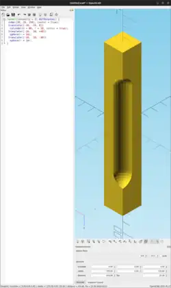
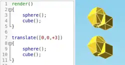
Usage examples:
render( convexity = 2 )
difference()
{ // stretch a cube vertically
cube([20, 20, 150], center = true);
// make a notch in one corner
translate([-10, -10, 0])
cylinder(h = 80, r = 10, center = true);
translate([-10, -10, +40])
sphere(r = 10);
translate([-10, -10, -40])
sphere(r = 10);
}
Surface() Object Module: Apply a Height Map
The Surface module draws a surface based on the Height map information given either as numbers in a text data file, or by interpreting the luminance of each pixel in a PNG image file (only).
The generated surface is normally drawn from the (0,0) origin in the +X,+Y quadrant. The extent of the drawn surface is either:
- data file - the number of columns and rows in the file
- image - the number of pixels in each direction of the image.
To make a surface of size (m,n) there must be n rows of numbers, with m values on each row.
Height values from an image file are massaged to the range of 0-100 and so will not have negative values, unless the invert option changes the sign of all the height values.
Height values are applied starting at the [0,0] corner. The column index and the X coordinate are both increased by one and the next value applied at the next position on the surface. Continue like this to the end of the row and then increase the Y coordinate, and the row index, by one as the row is completed. Repeat until all the rows are processed.
For a data file of size (m,n) the generated surface is grid of squares with the height value applied at the left-lower corner (as seen here). The n-th row of heights will be on the top vertices of the squares along the top edge of the surface:
^ [x,y+n] [x+m,y+n] | y [x,y] [x+m,y] [0,0] x-->
A one unit thick base is drawn downwards under the generated surface from the level of the smallest value in the data file, including when heights have negative values. This means that when least height value is zero the base will extend down to z=-1.
Parameters
- filename
- Required String. The filename may include an absolute or a relative path to the height map data file. There is no default so the .png extension must be explicitly given.
- center
- Optional Boolean, default=
falseto draw in the +X,+Y quadrant. Whentruethe surface is centered on the X-Y origin. - invert
- Optional Boolean, default=false. Limitation: Only applies to image based maps
. Inverts how the pixel values are interpreted into height values.[Note: Requires version 2015.03]
- convexity
- Integer, default=1. Higher values improve preview rendering of complex shapes. Limitation: Only used by OpenCSG Preview
Text Data Format
A text data height map is simply rows of whitespace separated, floating point numbers. The values may be written as integers, floating point with decimal fractions, or using exponential notation such as 1.25e2 for 125.
Hex values are not accepted but may not give a warning.
Consider a data file with n rows and m values on each, thus having size (m,n). The X position of each data point is given by their position along their row, and the Y by the row. The implicit indexing starts at the beginning of the file with the first row being at Y=0 and the first point on each row at X=0. The X and Y positions increment by one until X=m and Y=n, which means that the last row of values is the farthest edge of the generated surface.
The appearance of a hash sign ('#') as the first, non-whitespace character on a line marks it as a comment. A hash mark following numbers on a row cause a lexical fault making the data file unreadable.
Examples Using Data Map
//surface.scad surface(file = "surface.dat", center = true, convexity = 5); %translate([0,0,5]) cube([10,10,10], center = true);
The transparent cube shows the extent of the data space, and that the base extends downwards to Y=-1.
#surface.dat 10 9 8 7 6 5 5 5 5 5 9 8 7 6 6 4 3 2 1 0 8 7 6 6 4 3 2 1 0 0 7 6 6 4 3 2 1 0 0 0 6 6 4 3 2 1 1 0 0 0 6 6 3 2 1 1 1 0 0 0 6 6 2 1 1 1 1 0 0 0 6 6 1 0 0 0 0 0 0 0 3 1 0 0 0 0 0 0 0 0 3 0 0 0 0 0 0 0 0 0
Result:

One may use an application like Octave or Matlab to make a data file. This is a small Matlab script that superimposes two sine waves to create a 3D surface:
d = (sin(1:0.2:10)' * cos(1:0.2:10)) * 10;
save("-ascii", "example010.dat", "d");
The data file can then be used to draw the surface three ways:
//draw an instance of the surface
surface(file = "example010.dat", center = true);
//draw another instance, now rotated
translate(v = [70, 0, 0])
rotate(45, [0, 0, 1])
surface(file = "example010.dat", center = true);
// and two last instances, intersected
translate(v = [35, 60, 0])
intersection() {
surface(file = "example010.dat", center = true);
rotate(45, [0, 0, 1])
surface(file = "example010.dat", center = true);
}

Image Base Height Maps
[Note: Requires version 2015.03]
Heights are calculated using the linear luminance for the sRGB color space (Y = 0.2126R + 0.7152G + 0.0722B) at each pixel to derive a Grayscale value, which are further scaled to the range [0:100]. For an image with a color space between black (rgb=0,0,0) and white (rgb=1,1,1) the gray scale will be the full range.
For an image with a a narrower range of colors the gray scale is likewise reduced, and the minimum and maximum luminance in the color range set the lowest and highest limits, respectively, on the surface's heights.
Note also that no base is added below the surface as is done for a data file surface. Squares at Z=0, black, do have a surface filled in so the entire area of the surface is continuous.
Normally, with invert=false, the surface will be drawn upwards from the X-Y plane with black being z=0 increasing up to white=100. When invert=true the shape is still drawn starting at the X-Y plane, but now downwards to white=-100.
Currently only PNG (.png) images are supported and only the RGB channels are used. Specifically, the alpha channel is ignored.
Example Using Invert
// Example 3a - apply a scale to the surface scale([1, 1, 0.1]) surface(file = "smiley.png", center = true); scale([1, 1, 0.1]) surface(file = "smiley.png", center = true, invert = true);
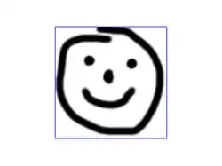
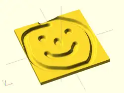
.png)
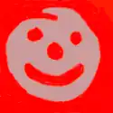
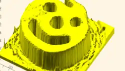
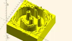
Note that the surfaces are above or, for the inverted surface, below, the X-Y plane, unlike Example 3
Example Grayscale Effects [Note: Requires version 2015.03]
surface(file = "BRGY-Grey.png", center = true, invert = false);
-
 PNG Test File
 -
 3D Surface
Search Function
The search() function is a general-purpose function to find one or more (or all) occurrences of a value or list of values in a vector, string or more complex list-of-list construct.
Search usage
- search( match_value , string_or_vector [, num_returns_per_match [, index_col_num ] ] );
Search arguments
- match_value
- Can be a single string value. Search loops over the characters in the string and searches for each one in the second argument. The second argument must be a string or a list of lists (this second case is not recommended). The search function does not search for substrings.
- Can be a single numerical value.
- Can be a list of values. The search function searches for each item on the list.
- To search for a list or a full string give the list or string as a single element list such as ["abc"] to search for the string "abc" (See Example 9) or [[6,7,8]] to search for the list [6,7,8]. Without the extra brackets, search looks separately for each item in the list.
- If match_value is boolean then search returns undef.
- string_or_vector
- The string or vector to search for matches.
- If match_value is a string then this should be a string and the string is searched for individual character matches to the characters in match_value
- If this is a list of lists, v=[[a0,a1,a2...],[b0,b1,b2,...],[c0,c1,c2,...],...] then search looks only at one index position of the sublists. By default this is position 0, so the search looks only at a0, b0, c0, etc. The index_col_num parameter changes which index is searched.
- If match_value is a string and this parameter is a list of lists then the characters of the string are tested against the appropriate index entry in the list of lists. However, if any characters fail to find a match a warning message is printed and that return value is excluded from the output (if num_returns_per_match is 1). This means that the length of the output is unpredictable.
- num_returns_per_match (default: 1)
- By default, search only looks for one match per element of match_value to return as a list of indices
- If num_returns_per_match > 1, search returns a list of lists of up to num_returns_per_match index values for each element of match_value.
- See Example 8 below.
- If num_returns_per_match = 0, search returns a list of lists of all matching index values for each element of match_value.
- See Example 6 below.
- index_col_num (default: 0)
- As noted above, when searching a list of lists, search looks only at one index position of each sublist. That index position is specified by index_col_num.
- See Example 5 below for a simple usage example.
Search usage examples
- See example023.scad included with OpenSCAD for a renderable example.
Index values return as list
| Example | Code | Result |
|---|---|---|
|
1 |
|
[0] |
|
2 |
|
[] |
|
3 |
|
[[0,4]] |
|
4 |
|
[[0,4]] (see also Example 6 below) |
Search on different column; return Index values
Example 5:
data= [ ["a",1],["b",2],["c",3],["d",4],["a",5],["b",6],["c",7],["d",8],["e",3] ]; echo(search(3, data)); // Searches index 0, so it doesn't find anything echo(search(3, data, num_returns_per_match=0, index_col_num=1));
Outputs:
ECHO: [] ECHO: [2, 8]
Search on list of values
Example 6: Return all matches per search vector element.
data= [ ["a",1],["b",2],["c",3],["d",4],["a",5],["b",6],["c",7],["d",8],["e",9] ];
search("abc", data, num_returns_per_match=0);
Returns:
[[0,4],[1,5],[2,6]]
Example 7: Return first match per search vector element; special case return vector.
data= [ ["a",1],["b",2],["c",3],["d",4],["a",5],["b",6],["c",7],["d",8],["e",9] ];
search("abc", data, num_returns_per_match=1);
Returns:
[0,1,2]
Example 8: Return first two matches per search vector element; vector of vectors.
data= [ ["a",1],["b",2],["c",3],["d",4],["a",5],["b",6],["c",7],["d",8],["e",9] ];
search("abce", data, num_returns_per_match=2);
Returns:
[[0,4],[1,5],[2,6],[8]]
Search on list of strings
Example 9:
lTable2=[ ["cat",1],["b",2],["c",3],["dog",4],["a",5],["b",6],["c",7],["d",8],["e",9],["apple",10],["a",11] ];
lSearch2=["b","zzz","a","c","apple","dog"];
l2=search(lSearch2,lTable2);
echo(str("Default list string search (",lSearch2,"): ",l2));
Returns
ECHO: "Default list string search (["b", "zzz", "a", "c", "apple", "dog"]): [1, [], 4, 2, 9, 3]"
Getting the right results
// workout which vectors get the results
v=[ ["O",2],["p",3],["e",9],["n",4],["S",5],["C",6],["A",7],["D",8] ];
//
echo(v[0]); // -> ["O",2]
echo(v[1]); // -> ["p",3]
echo(v[1][0],v[1][1]); // -> "p",3
echo(search("p",v)); // find "p" -> [1]
echo(search("p",v)[0]); // -> 1
echo(search(9,v,0,1)); // find 9 -> [2]
echo(v[search(9,v,0,1)[0]]); // -> ["e",9]
echo(v[search(9,v,0,1)[0]][0]); // -> "e"
echo(v[search(9,v,0,1)[0]][1]); // -> 9
echo(v[search("p",v,1,0)[0]][1]); // -> 3
echo(v[search("p",v,1,0)[0]][0]); // -> "p"
echo(v[search("d",v,1,0)[0]][0]); // "d" not found -> undef
echo(v[search("D",v,1,0)[0]][1]); // -> 8
Version() Function
There are two functions that obtain the applications version information.
- version()
- returns version as a vector of three numbers
[2011, 9, 23] - version_num()
- returns it as a number
20110923
parent_module(n) Function
$parent_modules is a special variable that holds the current depth of the instantiation stack.
The parent_module(n) function returns the name of the module n levels above the module currently at the top of the instantiation stack.
Parameters
- n
- non-negative integer, the index of the module to get the name of. The value gives the number of steps down the stack to the module of interest. This argument should not be greater than the current value of
$parent_modules.
The stack is constructed during the operation of a script, getting deeper as function or module calls create nested instances of modules, and reducing as deeper instances finish and return.
The definitions of named objects in the script(s) have nothing to do with the stack.
Example
module top() { // define an operator module
children();
}
module middle() { // define another operator module
children();
}
top()
middle() // top of the stack, the 0-th item
echo(parent_module(0)); // prints "middle"
top() // 1 step down the stack
middle()
echo(parent_module(1)); // prints "top"
assert()
[Note: Requires version 2019.05] see also Assertion (software development)
This is a syntactic element that may be used nearly anywhere in a script. It is not a function call, does not affect scope, and cannot have a child block using braces ( "{}" ).
Assert evaluates the condition which should normally be an expression giving a Boolean result.
When the result is false, the script halts and emits an error message to the console.
The default report is a string showing the expression and line number.
If the second argument is given it is appended to the message.
assert(condition) assert(condition, message)
Note that the appearance of assert() does not, by itself, form a statement and so no semi-colon (";") is needed to terminate it Parameters
- condition
- the expression given will be resolved to a Boolean true/false, if necessary using the rules for converting non-boolean values.
- message
- String to be appended to the message emitted when the assertion fails.
Examples
A call to assert(false); will halt the running script.
assert(false)
Emitting this message on the console
ERROR: Assertion 'false' failed in file assert_example1.scad, line 2
Checking Parameters
// Row must draw at least 3 spheres
module row(qty) {
assert(qty>= 3) // NOT the end of a statement
for (i = [1 : qty])
translate([i * 2, 0, 0]) sphere();
}
row(0);
// ERROR: Assertion '(qty > 0)' failed in file assert_example2.scad, line 3
In cases like this using the added message can show the user how the module is intended to be used. If the assert() could be changed to:
assert(qty > 0, "Quantity must be at least 3.");
the output is more useful:
// ERROR: Assertion '(qty>=0)': "Quantity must be at least 3./" failed in file assert_example3.scad, line 2
The qty parameter can be a floating value, but by its use in the for-loop it probably should not be.
The assertion can be expanded:
assert( is_num(qty) && qty >=3 )
to tighten the requirements on the input parameter
Checking Function Parameters Functions are limited to a single expression that returns a value. It is not possible to use additional if-the-else statements to test a function's given inputs but a nested ?: conditional statement avoids that restriction:
// set all letters to "lower case"
function lower(string) =
is_not_string( string ) ?
undef
: str_is_empty( string ) ?
""
: str_lower( string )
;
This method has the advantage that bad inputs do not halt execution, but some may prefer a stricter enforcement of a function's interface, thusly:
// set all letters to "lower case"
function lower(string) =
assert( ! is_string( string ) )
assert( string != "" )
str_lower( string ) // does the work
; // end of the function definition staement
If the lower() function is called with improper inputs the user will get immediate feedback.
Testing Features
To test a function that accumulates the values of an array we can set up test conditions that we know have to be correct
if(_NUMTEST_ENABLED) {
echo( "\ttesting cumsum_vec()" );
csv = [1,3,7,1];
vec=[ 10, 20, 30, 40 ];
echo( cs=cumsum_vec( csv ));
echo( cs=cumsum_vec( vec ));
}
assert( cumsum_vec( [1,3,7,1] ) == 12 );
assert( cumsum_vec( [10, 20, 30, 40] ) == 100 );
Chapter 7 -- User-Defined Functions and Modules
OpenSCAD User Manual/The OpenSCAD Language Users are encouraged to structure their programs by defining their own functions and modules.
Calculations that need to be done repeatedly may be encapsulated in functions, taking arguments and returning a value that may be used in an expression.
The normal operation of CSG, Constructive Solid Geometry, is to form complex shapes by the combination of primitive and derived shapes. When a complex design includes repeated instances of a component a custom Object Module may be defined. Likewise, when a sequence of operators is used repeatedly in a script it may be factored out to define an Operations Module.
Note: Names in OpenSCAD are case sensitive so test() is different from TEST() or Test()
Note: the terms "parameter" and "argument" are used interchangeably for the placeholder names used in the list of inputs to modules and functions
Definitions Limited By Scope
Functions, and modules of both types, may be named and defined locally, that is, inside a local scope. This means, of course, that calls made to those names from outside their scope will not find them and so produce a run-time error.
Function Arguments
The arguments named in the definition of a function or module must follow the rules for OpenSCAD names. They are local variables inside the function's scope.
Argument names should not be the same as any built-in or user-defined named object, special variable, or global variable as it could redefine the name in the scope of the function.
Arguments may be assigned a default value in this form
( arg1=10, arg2="default", arg3=false )
Note: arguments, like variables, are not typed so it is good to test positional arguments or to use assert()
Functions
Functions operate on their given parameters, or arguments, to calculate and return new values. The body of a function is a single expression so to define local variables the let() operator must be used.
- definition of a named function
function <name>( param=<default>, arg ) = expression;
- keyword
- literal "function"
- name
- the function name (see Rules on Names).
- (parameter,argument)
- Zero or more arguments Note: parameter and argument are synonyms .
- '='
- literal equals sign denoting the assignment operator
- value
- an expression that calculates a value which may be of any type.
- ';'
- literal semi-colon, end of definition statement
Function Literals
A function literal is a way to encapsulate a calculation in an object that can then be used in place of a literal value in an expression, function or module call, or even be assigned to a variable or returned by a function.
These objects are called anonymous functions, closures, or lambdas.
[Note: Requires version 2021.01]
- definition of a lambda function
function( param<default>, arg ) expression;
- keyword
- literal "function"
- (parameter,argument)
- Zero or more arguments, optionally with a default value Note: parameter and argument are synonyms .
- value
- an expression that calculates a value which may be of any type.
Note: the lack of a name and of the equals sign Function literals can be assigned to variables and passed around like any value. Calling the function uses the normal function call syntax with parenthesis.
func = function (x) x * x; echo(func(5)); // ECHO: 25
When called as part of an expression lambdas are calculated before other operators.
The following script defines three lambdas: the first is assigned to the variable "selector" which, when called, will create one of the two inner lambdas to return as its result:
// assign a lambda to variable "selector"
selector = function (which)
which == "add" ?
function (x) x + x // lambda for addition
: function (x) x * x; // and for multiplication
// display the value of "selector" for "add"
echo(selector("add")); // ECHO: function(x) ((x + x))
// call the function via selector to add 5+5
echo(selector("add")(5)); // ECHO: 10
// .. and for "mul"
echo(selector("mul")); // ECHO: function(x) ((x * x))
// call the function via selector to do 5 x 5
echo(selector("mul")(5)); // ECHO: 25
Using Functions
function trivial() = 5; // minimum and trivial
function func1(x=3) = 2*x+1;
function func2() = [1,2,3,4];
function func3(y=7) = (y==7) ? 5 : 2 ;
function func4(p0,p1,p2,p3) = [p0,p1,p2,p3];
echo(func0()); // 5
a = func1(); // 7
b = func1(5); // 11
echo(func2()); // [1, 2, 3, 4]
echo(func3(2), func3()); // 2, 5
z = func4(func0(), func1(), func2(), func3());
// [5, 7, [1, 2, 3, 4], 5]
translate([0, -4*func0(), 0])
cube([func0(), 2*func0(), func0()]);
// same as translate([0,-20,0]) cube([5,10,5]);
// example 2 creates for() range to give desired no of steps to cover range
function steps(start, no_steps, end) =
[start : (end-start)/(no_steps-1) : end];
echo(steps(10, 3, 5)); // [10 : -2.5 : 5]
for (i = steps(10, 3, 5)) echo(i); // 10 7.5 5
echo(steps(10, 3, 15)); // [10 : 2.5 : 15]
for (i = steps(10, 3, 15)) echo(i); // 10 12.5 15
echo(steps(0, 5, 5)); // [0 : 1.25 : 5]
for (i = steps(0, 5, 5)) echo(i); // 0 1.25 2.5 3.75 5
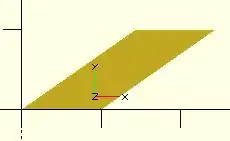
// example 3 rectangle with top pushed over, keeping same y
function rhomboid(x=1, y=1, angle=90)
= [[0,0],[x,0],
[x+x*cos(angle)/sin(angle),y],
[x*cos(angle)/sin(angle),y]];
echo (v1); v1 = rhomboid(10,10,35); // [[0, 0],
// [10, 0],
// [24.2815, 10],
// [14.2815, 10]]
polygon(v1);
polygon(rhomboid(10,10,35)); // alternate
//performing the same action with a module
module parallelogram(x=1,y=1,angle=90)
{polygon([[0,0],[x,0],
[x+x*cos(angle)/sin(angle),y],
[x*cos(angle)/sin(angle),y]]);};
parallelogram(10,10,35);
You can also use the let statement to create variables in a function:
function get_square_triangle_perimeter(p1, p2) =
let (hypotenuse = sqrt(p1*p1+p2*p2))
p1 + p2 + hypotenuse;
It can be used to store values in recursive functions. See the wikipedia page for more information on the general concept.
Recursive Functions
Recursive function calls are supported. Using the Conditional Operator "... ? ... : ... ", it is possible to ensure the recursion is terminated.
// recursion example: add all integers up to n
function add_up_to(n) = ( n==0 ?
0 :
n + add_up_to(n-1) );
There is a built-in recursion limit to prevent an application crash (a few thousands). If the limit is hit, you get an error like: ERROR: Recursion detected calling function ... .
For any tail-recursive function that calls itself, OpenSCAD is able to eliminate internally the recursion transforming it in an iterative loop.
The previous example code is not tail recursion, as the binary '+' can only execute when both its operand values are available. Its execution will therefore occur after the recursive call
add_up_to(n-1)has generated its second operand value.
However, the following is entitled to tail-recursion elimination:
// tail-recursion elimination example: add all integers up to n
function add_up_to(n, sum=0) =
n==0 ?
sum :
add_up_to(n-1, sum+n);
echo(sum=add_up_to(100000));
// ECHO: sum = 5.00005e+009
Tail-recursion elimination allows much higher recursion limits (up to 1000000).
Overwriting built-in functions
It is possible to overwrite the built-in functions. Note that definitions are handled first, so the evaluation does indeed return true for both echo() calls as those are evaluated in a later processing step.
| Source Code | Console output |
|---|---|
echo (sin(1));
function sin(x) = true;
echo (sin(1));
|
Compiling design (CSG Tree generation)...
ECHO: true
ECHO: true
Compiling design (CSG Products generation)...
|
Modules
Modules can be used to define objects or, using children(), define operators.
Once defined, modules are temporarily added to the language.
- module definition
module name ( parameters ) { actions }
- name
- Your name for this module. Try to pick something meaningful. Currently, valid names can only be composed of simple characters and underscores [a-zA-Z0-9_] and do not allow high-ASCII or Unicode characters.
- parameters
- Zero or more arguments. Parameters may be assigned default values, to use in case they are omitted in the call. Parameter names are local and do not conflict with external variables of the same name.
- actions
- Nearly any statement valid outside a module can be included within a module. This includes the definition of functions and other modules. Such functions and modules can be called only from within the enclosing module.
Variables can be assigned, but their scope is limited to within each individual use of the module. There is no mechanism in OpenSCAD for modules to return values to the outside. See Scope of variables for more details.
Object Modules
Object modules use one or more primitives, with associated operators, to define new objects.
In use, object modules are actions ending with a semi-colon ';'.
name ( parameter values );
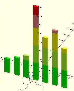
//example 1
translate([-30,-20,0])
ShowColorBars(Expense);
ColorBreak=[[0,""],
[20,"lime"], // upper limit of color range
[40,"greenyellow"],
[60,"yellow"],
[75,"LightCoral"],
[200,"red"]];
Expense=[16,20,25,85,52,63,45];
module ColorBar(value,period,range){ // 1 color on 1 bar
RangeHi = ColorBreak[range][0];
RangeLo = ColorBreak[range-1][0];
color( ColorBreak[range][1] )
translate([10*period,0,RangeLo])
if (value > RangeHi) cube([5,2,RangeHi-RangeLo]);
else if (value > RangeLo) cube([5,2,value-RangeLo]);
}
module ShowColorBars(values){
for (month = [0:len(values)-1], range = [1:len(ColorBreak)-1])
ColorBar(values[month],month,range);
}
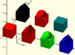
//example 2
module house(roof="flat",paint=[1,0,0]) {
color(paint)
if(roof=="flat") { translate([0,-1,0]) cube(); }
else if(roof=="pitched") {
rotate([90,0,0]) linear_extrude(height=1)
polygon(points=[[0,0],[0,1],[0.5,1.5],[1,1],[1,0]]); }
else if(roof=="domical") {
translate([0,-1,0]){
translate([0.5,0.5,1]) sphere(r=0.5,$fn=20); cube(); }
} }
house();
translate([2,0,0]) house("pitched");
translate([4,0,0]) house("domical",[0,1,0]);
translate([6,0,0]) house(roof="pitched",paint=[0,0,1]);
translate([0,3,0]) house(paint=[0,0,0],roof="pitched");
translate([2,3,0]) house(roof="domical");
translate([4,3,0]) house(paint=[0,0.5,0.5]);
//example 3
element_data = [[0,"","",0], // must be in order
[1,"Hydrogen","H",1.008], // indexed via atomic number
[2,"Helium", "He",4.003] // redundant atomic number to preserve your sanity later
];
Hydrogen = 1;
Helium = 2;
module coaster(atomic_number){
element = element_data[atomic_number][1];
symbol = element_data[atomic_number][2];
atomic_mass = element_data[atomic_number][3];
//rest of script
}
Operator Modules
Children()
Use of the children() module allows a module to access and operate on the child modules that may follow it in a statement.
name ( parameter values ){scope of operator}
Basically the children() command is used to apply modifications to objects that are focused by a scope:
module myModification() { rotate([0,45,0]) children(); }
myModification() // The modification
{ // Begin focus
cylinder(10,4,4); // First child
cube([20,2,2], true); // Second child
} // End focus
Children are indexed via integers from 0 to $children-1.
OpenSCAD sets $children to the total number of objects within the scope.
Objects grouped into a sub scope are treated as one child.
See example of separate children below and Scope of variables. Note that children(), echo() and empty block statements (including ifs) count as $children objects, even if no geometry is present (as of v2017.12.23).
children(); all children children(index); value or variable to select one child children([start : step : end]); select from start to end incremented by step children([start : end]); step defaults to 1 or -1 children([vector]); selection of several children
Deprecated child() module
Up to release 2013.06 the now deprecated child() module was used instead. This can be translated to the new children() according to the table:
| up to 2013.06 | 2014.03 and later |
|---|---|
| child() | children(0) |
| child(x) | children(x) |
| for (a = [0:$children-1]) child(a) | children([0:$children-1]) |
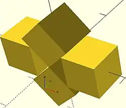
Examples
//Use all children
module move(x=0,y=0,z=0,rx=0,ry=0,rz=0)
{ translate([x,y,z])rotate([rx,ry,rz]) children(); }
move(10) cube(10,true);
move(-10) cube(10,true);
move(z=7.07, ry=45)cube(10,true);
move(z=-7.07,ry=45)cube(10,true);

//Use only the first child, multiple times
module lineup(num, space) {
for (i = [0 : num-1])
translate([ space*i, 0, 0 ]) children(0);
}
lineup(5, 65){ sphere(30);cube(35);}
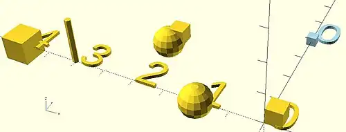
//Separate action for each child
module SeparateChildren(space){
for ( i= [0:1:$children-1]) // step needed in case $children < 2
translate([i*space,0,0]) {children(i);text(str(i));}
}
SeparateChildren(-20){
cube(5); // 0
sphere(5); // 1
translate([0,20,0]){ // 2
cube(5);
sphere(5);
}
cylinder(15); // 3
cube(8,true); // 4
}
translate([0,40,0])color("lightblue")
SeparateChildren(20){cube(3,true);}
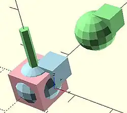
//Multiple ranges
module MultiRange(){
color("lightblue") children([0:1]);
color("lightgreen")children([2:$children-2]);
color("lightpink") children($children-1);
}
MultiRange()
{
cube(5); // 0
sphere(5); // 1
translate([0,20,0]){ // 2
cube(5);
sphere(5);
}
cylinder(15); // 3
cube(8,true); // 4
}
Further module examples
- Objects
module arrow(){
cylinder(10);
cube([4,.5,3],true);
cube([.5,4,3],true);
translate([0,0,10]) cylinder(4,2,0,true);
}
module cannon(){
difference(){union()
{sphere(10);cylinder(40,10,8);} cylinder(41,4,4);
} }
module base(){
difference(){
cube([40,30,20],true);
translate([0,0,5]) cube([50,20,15],true);
} }
- Operators
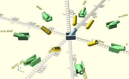
module aim(elevation,azimuth=0)
{ rotate([0,0,azimuth])
{ rotate([0,90-elevation,0]) children(0);
children([1:1:$children-1]); // step needed in case $children < 2
} }
aim(30,20)arrow();
aim(35,270)cannon();
aim(15){cannon();base();}
module RotaryCluster(radius=30,number=8)
for (azimuth =[0:360/number:359])
rotate([0,0,azimuth])
translate([radius,0,0]) { children();
translate([40,0,30]) text(str(azimuth)); }
RotaryCluster(200,7) color("lightgreen") aim(15){cannon();base();}
rotate([0,0,110]) RotaryCluster(100,4.5) aim(35)cannon();
color("LightBlue")aim(55,30){cannon();base();}
Recursive Modules
Like functions, modules may contain recursive calls. However, there is no tail-recursion elimination for recursive modules.
The code below generates a crude model of a tree. Each tree branch is itself a modified version of the tree and produced by recursion. Be careful to keep the recursion depth (branching) n below 7 as the number of primitives and the preview time grow exponentially.
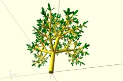
module simple_tree(size, dna, n) {
if (n > 0) {
// trunk
cylinder(r1=size/10, r2=size/12, h=size, $fn=24);
// branches
translate([0,0,size])
for(bd = dna) {
angx = bd[0];
angz = bd[1];
scal = bd[2];
rotate([angx,0,angz])
simple_tree(scal*size, dna, n-1);
}
}
else { // leaves
color("green")
scale([1,1,3])
translate([0,0,size/6])
rotate([90,0,0])
cylinder(r=size/6,h=size/10);
}
}
// dna is a list of branching data bd of the tree:
// bd[0] - inclination of the branch
// bd[1] - Z rotation angle of the branch
// bd[2] - relative scale of the branch
dna = [ [12, 80, 0.85], [55, 0, 0.6],
[62, 125, 0.6], [57, -125, 0.6] ];
simple_tree(50, dna, 5);
Another example of recursive module may be found in Tips and Tricks
Overwriting built-in modules
It is possible to overwrite the built-in modules.
A simple, but pointless example would be:
module sphere(){
square();
}
sphere();
Note that the built-in sphere module can not be called when over written.
A more sensible way to use this language feature is to overwrite the 3D primitives with extruded 2D-primitives. This allows additional customization of the default parameters and adding additional parameters.
Chapter 8 -- Debugging aids
OpenSCAD User Manual/The OpenSCAD Language
Modifier characters are used to change the appearance or behaviors of child nodes. They are particularly useful in debugging where they can be used to highlight specific objects, or include or exclude them from rendering.
Advanced concept
OpenSCAD uses different libraries to implement capabilities, and this can introduce some inconsistencies to the F5 preview behavior of transformations. Traditional transforms (translate, rotate, scale, mirror & multimatrix) are performed using OpenGL in preview, while other more advanced transforms, such as resize, perform a CGAL operation, behaving like a CSG operation affecting the underlying object, not just transforming it. In particular this can affect the display of modifier characters, specifically "#" and "%", where the highlight may not display intuitively, such as highlighting the pre-resized object, but highlighting the post-scaled object.
Note: The color changes triggered by character modifiers appear only in "Compile" mode, not "Compile and Render (CGAL)" mode. (As per the color section.)
Background modifier
Ignore this subtree for the normal rendering process and draw it in transparent gray (all transformations are still applied to the nodes in this tree).
Because the marked subtree is completely ignored, it might have unexpected effects in case it's used, for example, with the first object in a difference(). In that case this object is rendered in transparent gray, but it is not used as the base for the difference()!
Usage
% { ... }
Example
difference() {
cylinder (h = 12, r=5, center = true, $fn=100);
// first object to be subtracted
rotate ([90,0,0]) cylinder (h = 15, r=1, center = true, $fn=100);
// second object to be subtracted
%rotate ([0,90,0]) cylinder (h = 15, r=3, center = true, $fn=100);
}
Example output
.png)
.png)
.png)
Debug modifier
Use this subtree as usual in the rendering process but also draw it unmodified in transparent pink.
Usage
# { ... }
Example
difference() {
// start objects
cylinder (h = 12, r=5, center = true, $fn=100);
// first object to be subtracted
#rotate ([90,0,0]) cylinder (h = 15, r=1, center = true, $fn=100);
// second object to be subtracted
#rotate ([0,90,0]) cylinder (h = 15, r=3, center = true, $fn=100);
}
Example output
.png)
.png)
Root modifier
Ignore the rest of the design and use this subtree as design root.
Usage
! { ... }
Example
difference() {
cube(10, center = true);
translate([0, 0, 5]) {
!rotate([90, 0, 0]) {
#cylinder(r = 2, h = 20, center = true, $fn = 40);
}
}
}
Example output
.png)
.png)
As shown in the example output with the root modifier active, the rotate() is executed as it's part of the subtree marked with the root modifier, but the translate() has no effect.
Disable modifier
Simply ignore this entire subtree.
Usage
* { ... }
Example
difference() {
cube(10, center = true);
translate([0, 0, 5]) {
rotate([0, 90, 0]) {
cylinder(r = 2, h = 20, center = true, $fn = 40);
}
*rotate([90, 0, 0]) {
#cylinder(r = 2, h = 20, center = true, $fn = 40);
}
}
}
Example output
.png)
.png)
The disable modifier allows you to comment out one or multiple subtrees. Compared to using the usual line or multi-line comments, it's aware of the hierarchical structure, which makes it easier to disable even larger trees without the need to search for the end of the subtree.
Echo statements
This function prints the contents to the compilation window (aka Console). Useful for debugging code. Also see the String function str().
Numeric values are rounded to 5 significant digits.
It can be handy to use 'variable=variable' as the expression to easily label the variables, see the example below.
Usage examples:
my_h=50;
my_r=100;
echo("This is a cylinder with h=", my_h, " and r=", my_r);
echo(my_h=my_h,my_r=my_r); // shortcut
cylinder(h=my_h, r=my_r);
Shows in the Console as
ECHO: "This is a cylinder with h=", 50, " and r=", 100 ECHO: my_h = 50, my_r = 100
Chapter 9 -- External libraries and code files
OpenSCAD User Manual/The OpenSCAD Language
Use and Include
For including code from external files in OpenSCAD, there are two commands available:
include <filename>acts as if the contents of the included file were written in the including file, anduse <filename>imports modules and functions, but does not execute any commands other than those definitions.
Library files are searched for in the same folder as the design was opened from, in the library folder of the OpenSCAD installation, and in folders given by the OPENSCADPATH environment variable. You can use a relative path specification to either. If they lie elsewhere you must give the complete path. Newer versions have predefined user libraries, see the OpenSCAD_User_Manual/Libraries page, which also documents a number of library files included in OpenSCAD.
Wildcards (e.g. include <MCAD/*.scad>) can not be used to include multiple files.
include <filename>
When file A includes file B, it is almost exactly as if B was dropped at that point in A. Everything in B is visible to A, and everything in A is visible to B.
Variables in included files
Generally, a particular instance of an OpenSCAD variable has only one value; it cannot be set to one value and then reset to another value. Attempting to change the value of a variable triggers a warning; if the warning is ignored then the last value assigned is used throughout its entire life. (See the Variables section for more information.)
Inclusion is a special exception to this rule. If included file B defines a variable, and main file A subsequently assigns a value to it, the warning that would normally be triggered is suppressed; the definition from file A is used throughout the life of the variable.
This behavior allows a library file to define a default value for a variable, and the main file to override that default.
B.scad
v = 1;
A.scad
include <B.scad> v = 5; echo(v=v);
Produces the following without any warning:
ECHO: v = 5
Caution: Order of Execution
The assignment by A is executed as if it was located at the original assignment in B. This can be an issue if the expression is dependent on other variables.
B.scad
a = 1; b = 2;
A.scad
include <B.scad> a = b + 1; echo(a=a, b=b);
fails, producing
WARNING: Ignoring unknown variable "b" in file a.scad, line 2 WARNING: undefined operation (undefined + number) in file a.scad, line 2 ECHO: a = undef, b = 2
var = include <filename>;
Because include is functionally equivalent to dropping an included file into the spot in the parent file where the include statement appeared (replacing the include statement with the new file) it is possible to assign data in an external file to a local variable name.
For example, suppose the file data.txt contains a comma-delimited list of numbers:
8, 6, 3, 8, 6, 4, 5, 99, 8, 1, 3, 5
Then in OpenSCAD, putting the include inside array brackets imports the data as an OpenSCAD array:
numlist = [ include <data.txt> ]; echo(numlist);
produces:
ECHO: [8, 6, 3, 8, 6, 4, 5, 99, 8, 1, 3, 5]
One would think that it's possible to import CSV data in a similar fashion, by knowing the number of columns in the CSV file in advance, and split the array into a list of row arrays, but this wouldn't work. CSV allows for empty data between commas, which are ignored by OpenSCAD, causing differences in the lengths of each row. It is best to preprocess a CSV file into a more compatible format before including it.
Another example: suppose the file cube.poly contains an array describing a polyhedron for a cube, with a list of 8 vertices followed by a list of 6 faces.
[
[ // vertices
[37.5,67.5,0], [37.5,42.5,0], [12.5,42.5,0], [12.5,67.5,0],
[37.5,67.5,25], [12.5,67.5,25], [12.5,42.5,25], [37.5,42.5,25]
],
[ // faces
[3,2,1,0], [7,6,5,4], [1,7,4,0], [2,6,7,1], [3,5,6,2], [5,3,0,4]
]
]
Because include replaces itself with the included file, one can assign the include to a variable name:
cube_poly = include <cube.poly>; vertices = cube_poly[0]; faces = cube_poly[1]; polyhedron(vertices, faces);
When using this trick to assign the contents of an included file to a variable name, avoid doing this with .scad files. Your data files should have some other extension, because the included file should contain data rather than OpenSCAD source code.
use <filename>
When file A uses file B:
- A can see B's modules and functions.
- A cannot see B's global variables.
- B cannot see A's global variables.
- B cannot see A's modules and functions.
- B's top-level module invocations are not executed.
- B's top-level assignments are executed on every call from A to B. (This can be useful if they are dependent on $ variables defined by A, or can be a performance problem.)
use <filename> is allowed only at the top level of a file.
Example "Ring Library"
A library file for generating rings might look like this:
ring.scad:
module ring(r1, r2, h) {
difference() {
cylinder(r = r1, h = h);
translate([ 0, 0, -1 ]) cylinder(r = r2, h = h+2);
}
}
ring(5, 4, 10);
Including the library using
include <ring.scad> rotate([90, 0, 0]) ring(10, 1, 1);
would result in the example ring being shown in addition to the rotated ring, but
use <ring.scad> rotate([90, 0, 0]) ring(10, 1, 1);
shows only the rotated ring.
Additional Notes
Directory separators
Windows and Linux/Mac use different separators for directories. Windows uses \, e.g. directory\file.ext, while the others use /, e.g. directory/file.ext. This could lead to cross platform issues. However OpenSCAD on Windows correctly handles the use of /, so using / in all include or use statements works on all platforms.
Nested Include and Use
OpenSCAD executes nested calls to include and use. There is one caveat to this, that use brings functions and modules only into the local file context. As a result, nested calls to use have no effect on the environment of the base file; the child use call works in the parent use context, but the modules and functions so imported fall out of context before they are seen by the base context.
Importing 3D Solids
In older versions of the application files of each format were imported using a module specific to it. These older modules are deprecated in newer versions but are still documented in this page.
Currently the import() Object Module processes each type of file according to its file extension to instantiate imported objects. [Note: Requires version 2015.03]
There are some other, purpose specific, import methods in the app:
- A '.csg' geometry file
- may be imported by an
include <filename.csg>statement. - A '.png' image
- The import image option of the surface() object module may be used to apply a height map to a surface.
- data in a text file
- The import numeric data of the surface() object module may also be used to apply a height map.
- data in a JSON file
- The import() function may can read structured data into an object that can then be processed by a script.
Include <"filename.csg">
A .csg format file is a type of geometry file exported from OpenSCAD using a subset of its programming language.
As such the shapes described by it may be imported into a program using the include <filename.csg> statement.
Import() Object Module
This is an Object Module that imports geometry for use in the script. The extension on the filename informs the module as to which input processor to use.
The import() function is a separate component for bringing in structured data from a JSON file.
Parameters
- file
- A string containing a filename and extension of form "filename.ext". The location of the file is the same as the script's file. Refer to the File System Issues page for other file path options and platform specific information.
filename- deprecated - a filename of form "filename.ext". Use "file" parameter.
- origin
- vector of form [xcoord,ycoord]
- scale
- number. A scale factor to apply to the model
- width
- number
- height
- number
- dpi
- non-negative integer >= 0.001. The Dots Per Inch value is used importing a SVG or DXF file to correctly size the generated geometry.
- center
- Boolean. When true the object is centered in the X-Y plane at the origin. [Note: Requires version Development snapshot]
- convexity
- non-negative integer. The convexity parameter specifies the maximum number of front sides (or back sides) a ray intersecting the object might penetrate. This parameter is needed only for correctly displaying the object in OpenCSG preview mode and has no effect on the polyhedron rendering. Optional.
- id
- String. For SVG import only, the id of an element or group to import. Optional. [Note: Requires version Development snapshot]
- layer
- For DXF and SVG import only, specify a specific layer to import. Optional.
layername- [Deprecated: layername will be removed in a future release. Use layer instead]
- $fn
- Number, default 0. The number of polygon segments to use when converting circles, arcs, and curves to polygons. [Note: Requires version Development snapshot]
- $fa
- Number, default 12. The minimum angle step to use when converting circles and arcs to polygons. [Note: Requires version Development snapshot]
- $fs
- Number, default 2. The minimum segment length to use when converting circles and arcs to polygons. [Note: Requires version Development snapshot]
3D Geometry Formats
There is a concise comparison of the commonly used file formats in 3D printing on the AnyCubic website that may be of interest.
These are the file formats recognized by import():
- OBJ
- OBJect data file by Wavefront
- AMF
- Additive Manufacturing Files include color, texture, and other meta data in addition to a 3D polygonal geometry but is deprecated as it has not achieved much acceptance in the industry.
- 3MF
- 3D Manufacturing Format XML data file
- CSG
- solid geometry format of OpenSCAD programming language
- STL
- STereoLithography file format by 3D Systems for describing polygons in a 3D coordinate space. Replaced by Additive Manufacturing Format (.amf)
- OFF
- Object File Format
- NEF3
- a CGAL geometry data format from a Nef Polygon object (ref section 15.6). It is used mostly by the OpenSCAD dev group as a debugging tool when building test cases for upstream reporting to CGAL.
2D Geometry Formats
Shapes drawn in two dimensional formats may also be imported by the import() module, as documented in the Import 2D page.
Image Formats
- PNG
- Portable Network Graphics image file. As already mentioned, the surface() method is able to derive a gray scale value from each pixel to apply to a surface as a height map.
import() Function - JSON only
[Note: Requires version Development snapshot]
This function returns an object with the structured data from a valid JSON file. Although it has the same name as the import() Module it is functionally separate in that it may only be used in an assignment statement and may not be the target action of an Operator Module.
/* "people.json" contains:
{"people":[{"name":"Helen", "age":19}, {"name":"Chris", "age":32}]}
*/
pf=import( file = "people.json" );
echo(pf);
people = pf.people;
for( p=people) {
echo(str( p.name, ": ", p.age));
}
or even
people = import( file = "people.json" ).people;
for( p=people) {
echo(str( p.name, ": ", p.age));
}
both of which give the data about Helen and Chris:
ECHO: { people = [{ age = 19; name = "Helen"; }, { age = 32; name = "Chris"; }]; }
ECHO: "Helen: 19"
ECHO: "Chris: 32"
Surface() Object Module: Apply a Height Map
The Surface module draws a surface based on the Height map information given either as numbers in a text data file, or by interpreting the luminance of each pixel in a PNG image file (only).
The generated surface is normally drawn from the (0,0) origin in the +X,+Y quadrant. The extent of the drawn surface is either:
- data file - the number of columns and rows in the file
- image - the number of pixels in each direction of the image.
To make a surface of size (m,n) there must be n rows of numbers, with m values on each row.
Height values from an image file are massaged to the range of 0-100 and so will not have negative values, unless the invert option changes the sign of all the height values.
Height values are applied starting at the [0,0] corner. The column index and the X coordinate are both increased by one and the next value applied at the next position on the surface. Continue like this to the end of the row and then increase the Y coordinate, and the row index, by one as the row is completed. Repeat until all the rows are processed.
For a data file of size (m,n) the generated surface is grid of squares with the height value applied at the left-lower corner (as seen here). The n-th row of heights will be on the top vertices of the squares along the top edge of the surface:
^ [x,y+n] [x+m,y+n] | y [x,y] [x+m,y] [0,0] x-->
A one unit thick base is drawn downwards under the generated surface from the level of the smallest value in the data file, including when heights have negative values. This means that when least height value is zero the base will extend down to z=-1.
Parameters
- filename
- Required String. The filename may include an absolute or a relative path to the height map data file. There is no default so the .png extension must be explicitly given.
- center
- Optional Boolean, default=
falseto draw in the +X,+Y quadrant. Whentruethe surface is centered on the X-Y origin. - invert
- Optional Boolean, default=false. Limitation: Only applies to image based maps
. Inverts how the pixel values are interpreted into height values.[Note: Requires version 2015.03]
- convexity
- Integer, default=1. Higher values improve preview rendering of complex shapes. Limitation: Only used by OpenCSG Preview
Text Data Format
A text data height map is simply rows of whitespace separated, floating point numbers. The values may be written as integers, floating point with decimal fractions, or using exponential notation such as 1.25e2 for 125.
Hex values are not accepted but may not give a warning.
Consider a data file with n rows and m values on each, thus having size (m,n). The X position of each data point is given by their position along their row, and the Y by the row. The implicit indexing starts at the beginning of the file with the first row being at Y=0 and the first point on each row at X=0. The X and Y positions increment by one until X=m and Y=n, which means that the last row of values is the farthest edge of the generated surface.
The appearance of a hash sign ('#') as the first, non-whitespace character on a line marks it as a comment. A hash mark following numbers on a row cause a lexical fault making the data file unreadable.
Examples Using Data Map
//surface.scad surface(file = "surface.dat", center = true, convexity = 5); %translate([0,0,5]) cube([10,10,10], center = true);
The transparent cube shows the extent of the data space, and that the base extends downwards to Y=-1.
#surface.dat 10 9 8 7 6 5 5 5 5 5 9 8 7 6 6 4 3 2 1 0 8 7 6 6 4 3 2 1 0 0 7 6 6 4 3 2 1 0 0 0 6 6 4 3 2 1 1 0 0 0 6 6 3 2 1 1 1 0 0 0 6 6 2 1 1 1 1 0 0 0 6 6 1 0 0 0 0 0 0 0 3 1 0 0 0 0 0 0 0 0 3 0 0 0 0 0 0 0 0 0
Result:
One may use an application like Octave or Matlab to make a data file. This is a small Matlab script that superimposes two sine waves to create a 3D surface:
d = (sin(1:0.2:10)' * cos(1:0.2:10)) * 10;
save("-ascii", "example010.dat", "d");
The data file can then be used to draw the surface three ways:
//draw an instance of the surface
surface(file = "example010.dat", center = true);
//draw another instance, now rotated
translate(v = [70, 0, 0])
rotate(45, [0, 0, 1])
surface(file = "example010.dat", center = true);
// and two last instances, intersected
translate(v = [35, 60, 0])
intersection() {
surface(file = "example010.dat", center = true);
rotate(45, [0, 0, 1])
surface(file = "example010.dat", center = true);
}
Image Base Height Maps
[Note: Requires version 2015.03]
Heights are calculated using the linear luminance for the sRGB color space (Y = 0.2126R + 0.7152G + 0.0722B) at each pixel to derive a Grayscale value, which are further scaled to the range [0:100]. For an image with a color space between black (rgb=0,0,0) and white (rgb=1,1,1) the gray scale will be the full range.
For an image with a a narrower range of colors the gray scale is likewise reduced, and the minimum and maximum luminance in the color range set the lowest and highest limits, respectively, on the surface's heights.
Note also that no base is added below the surface as is done for a data file surface. Squares at Z=0, black, do have a surface filled in so the entire area of the surface is continuous.
Normally, with invert=false, the surface will be drawn upwards from the X-Y plane with black being z=0 increasing up to white=100. When invert=true the shape is still drawn starting at the X-Y plane, but now downwards to white=-100.
Currently only PNG (.png) images are supported and only the RGB channels are used. Specifically, the alpha channel is ignored.
Example Using Invert
// Example 3a - apply a scale to the surface scale([1, 1, 0.1]) surface(file = "smiley.png", center = true); scale([1, 1, 0.1]) surface(file = "smiley.png", center = true, invert = true);
Note that the surfaces are above or, for the inverted surface, below, the X-Y plane, unlike Example 3
Example Grayscale Effects [Note: Requires version 2015.03]
surface(file = "BRGY-Grey.png", center = true, invert = false);
-
PNG Test File
-
3D Surface